
Recap: k-Nearest Neighbor#
Building the model consists only of storing the training dataset.
To make a prediction, the algorithm finds the k closest data points in the training dataset
Classification: predict the most frequent class of the k neighbors
Regression: predict the average of the values of the k neighbors
Both can be weighted by the distance to each neighbor
Main hyper-parameters:
Number of neighbors (k). Acts as a regularizer.
Choice of distance function (e.g. Euclidean)
Weighting scheme (uniform, distance,…)
Model:
Representation: Store training examples (e.g. in KD-tree)
Typical loss functions:
Classification: Accuracy (Zero-One Loss)
Regression: Root mean squared error
Optimization: None (no model parameters to tune)
# Auto-setup when running on Google Colab
import os
if 'google.colab' in str(get_ipython()) and not os.path.exists('/content/master'):
    !git clone -q https://github.com/ML-course/master.git /content/master
    !pip install -rq master/requirements_colab.txt
    %cd master/notebooks

# Global imports and settings
%matplotlib inline
from preamble import *
interactive = True # Set to True for interactive plots
if interactive:
    fig_scale = 1.5
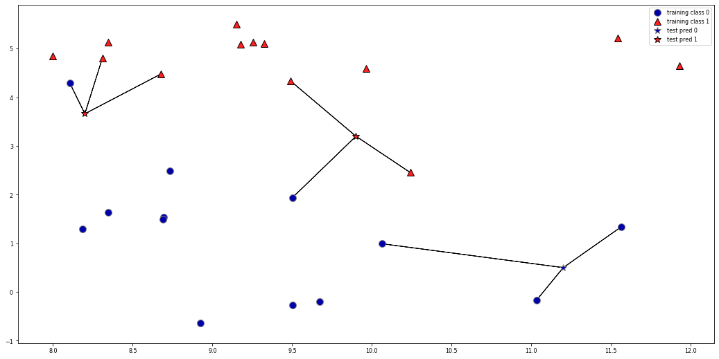
k-Nearest Neighbor Classification#
k=1: look at nearest neighbor only: likely to overfit
k>1: do a vote and return the majority (or a confidence value for each class)
plt.rcParams["figure.figsize"] = (12*fig_scale,6*fig_scale)
mglearn.plots.plot_knn_classification(n_neighbors=3)
Analysis#
We can plot the prediction for each possible input to see the decision boundary
from sklearn.neighbors import KNeighborsClassifier
X, y = mglearn.datasets.make_forge()
fig, axes = plt.subplots(1, 3, figsize=(10*fig_scale, 3*fig_scale))

for n_neighbors, ax in zip([1, 3, 9], axes):
    clf = KNeighborsClassifier(n_neighbors=n_neighbors).fit(X, y)
    mglearn.plots.plot_2d_separator(clf, X, fill=True, eps=0.5, ax=ax, alpha=.4)
    mglearn.discrete_scatter(X[:, 0], X[:, 1], y, ax=ax)
    ax.set_title("{} neighbor(s)".format(n_neighbors))
    ax.set_xlabel("feature 0")
    ax.set_ylabel("feature 1")
_ = axes[0].legend(loc=3)
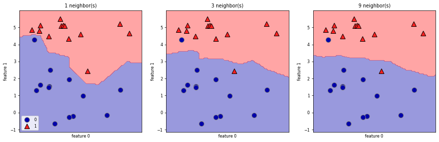
Using few neighbors corresponds to high model complexity (left), and using many neighbors corresponds to low model complexity and smoother decision boundary (right).
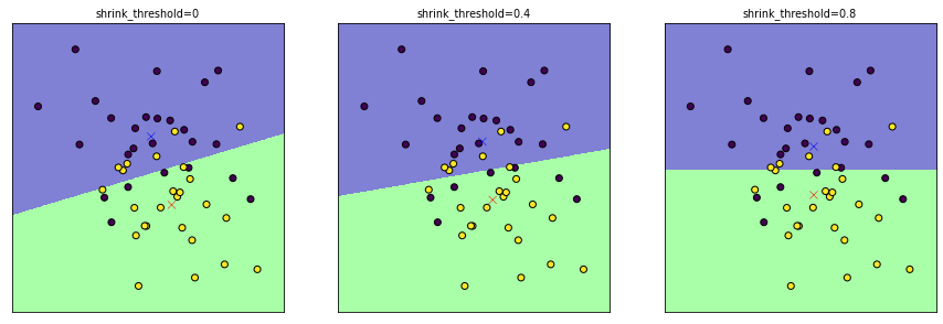
Nearest Shrunken Centroid#
Nearest Centroid: Represents each class by the centroid of its members.
Parameteric model (while kNN is non-parametric)
Regularization is possible with the
shrink_thresholdparameterShrinks (scales) each feature value by within-class variance of that feature
Soft thresholding: if feature value falls below threshold, it is set to 0
Effectively removes (noisy) features
from sklearn.neighbors import NearestCentroid
from sklearn.datasets import make_blobs
fig, axes = plt.subplots(1, 3, figsize=(10*fig_scale, 5*fig_scale))
thresholds = [0, 0.4, .8]
X, y = make_blobs(centers=2, cluster_std=2, random_state=0, n_samples=50)

for threshold, ax in zip(thresholds, axes):
    ax.set_title(f"shrink_threshold={threshold}")
    nc = NearestCentroid(shrink_threshold=threshold)
    nc.fit(X, y)
    ax.scatter(X[:, 0], X[:, 1], c=y, edgecolor='k')
    mglearn.tools.plot_2d_classification(nc, X, alpha=.5, ax=ax)
    ax.scatter(nc.centroids_[:, 0], nc.centroids_[:, 1], c=['b', 'r'], s=50, marker='x')
    ax.set_aspect("equal")
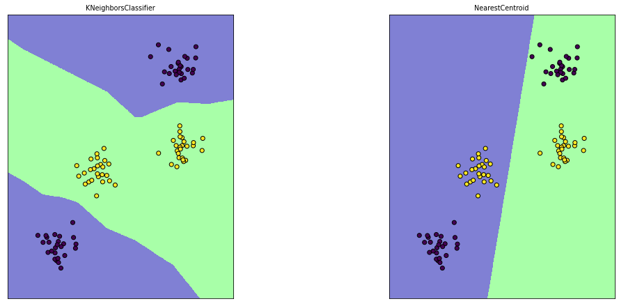
Note: Nearest Centroid suffers when the data is not ‘convex’
X, y = make_blobs(centers=4, random_state=8)
y = y % 2

knn = KNeighborsClassifier(n_neighbors=1).fit(X, y)
nc = NearestCentroid().fit(X, y)

plt.figure
fig, axes = plt.subplots(1, 2, figsize=(12*fig_scale, 5*fig_scale))
for est, ax in [(knn, axes[0]), (nc, axes[1])]:
    ax.scatter(X[:, 0], X[:, 1], c=y, edgecolor='k')

    ax.set_title(est.__class__.__name__)
    mglearn.tools.plot_2d_classification(est, X, alpha=.5, ax=ax)
    ax.set_aspect("equal")
Scalability#
With \(n\) = nr examples and \(p\) = nr features
Nearest shrunken threshold
Fit: \(O(n \cdot p)\)
Memory: \(O(\text{nrclasses} \cdot p)\)
Predict: \(O(\text{nrclasses} \cdot p)\)
Nearest neighbors (naive)
Fit: \(0\)
Memory: \(O(n \cdot p)\)
Predict: \(O(n \cdot p)\)
Nearest neighbors (with KD trees)
Fit: \(O(p \cdot n \log n)\)
Memory: \(O(n \cdot p)\)
Predict: \(O(k \cdot \log n)\)
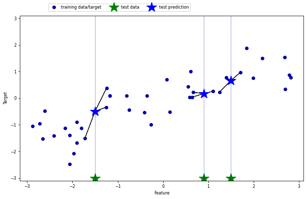
k-Neighbors Regression#
k=1: return the target value of the nearest neighbor (overfits easily)
k>1: return the mean of the target values of the k nearest neighbors
mglearn.plots.plot_knn_regression(n_neighbors=3)
Analysis#
We can again output the predictions for each possible input, for different values of k.
from sklearn.neighbors import KNeighborsRegressor
from sklearn.model_selection import train_test_split

# split the wave dataset into a training and a test set
X, y = mglearn.datasets.make_wave(n_samples=40)
X_train, X_test, y_train, y_test = train_test_split(X, y, random_state=0)

fig, axes = plt.subplots(1, 3, figsize=(15*fig_scale, 4*fig_scale))
# create 1000 data points, evenly spaced between -3 and 3
line = np.linspace(-3, 3, 1000).reshape(-1, 1)
for n_neighbors, ax in zip([1, 3, 9], axes):
    # make predictions using 1, 3 or 9 neighbors
    reg = KNeighborsRegressor(n_neighbors=n_neighbors)
    reg.fit(X_train, y_train)
    ax.plot(line, reg.predict(line))
    ax.plot(X_train, y_train, '^', c=mglearn.cm2(0), markersize=8)
    ax.plot(X_test, y_test, 'v', c=mglearn.cm2(1), markersize=8)

    ax.set_title(
        "{} neighbor(s)\n train score: {:.2f} test score: {:.2f}".format(
            n_neighbors, reg.score(X_train, y_train),
            reg.score(X_test, y_test)))
    ax.set_xlabel("Feature")
    ax.set_ylabel("Target")
_ = axes[0].legend(["Model predictions", "Training data/target",
                "Test data/target"], loc="best")
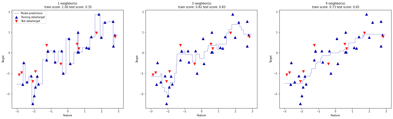
We see that again, a small k leads to an overly complex (overfitting) model, while a larger k yields a smoother fit.
kNN: Strengths, weaknesses and parameters#
Easy to understand, works well in many settings
Training is very fast, predicting is slow for large datasets
Bad at high-dimensional and sparse data (curse of dimensionality)
Nearest centroid is a useful parametric alternative, but only if data is (near) linearly separable.