Machine Learning in Python

# General imports
%matplotlib inline
import numpy as np
import pandas as pd
import matplotlib.pyplot as plt

Machine Learning in Python#

Joaquin Vanschoren, Eindhoven University of Technology

Why Python?#

Many data-heavy applications are now developed in Python
Highly readable, less complexity, fast prototyping
Easy to offload number crunching to underlying C/Fortran/…
Easy to install and import many rich libraries
- numpy: efficient data structures
- scipy: fast numerical recipes
- matplotlib: high-quality graphs
- scikit-learn: machine learning algorithms
- tensorflow: neural networks
- …

Numpy, Scipy, Matplotlib#

We’ll illustrate these with a practical example
Many good tutorials online

from scipy.stats import gamma
np.random.seed(3)  # to reproduce the data

def gen_web_traffic_data():
    '''
    This function generates some fake data that first shows a weekly pattern 
    for a couple weeks before it grows exponentially.
    '''
    # 31 days, 24 hours
    x = np.arange(1, 31*24)
    
    # Sine wave with weekly rhythm + noise + exponential increase
    y = np.array(200*(np.sin(2*np.pi*x/(7*24))), dtype=np.float32)
    y += gamma.rvs(15, loc=0, scale=100, size=len(x))
    y += 2 * np.exp(x/100.0)
    y = np.ma.array(y, mask=[y<0])

    return x, y

def plot_web_traffic(x, y, models=None, mx=None, ymax=None):
    '''
    Plot the web traffic (y) over time (x). 
    
    If models is given, it is expected to be a list fitted models,
    which will be plotted as well (used later).
    '''
    plt.figure(figsize=(12,6), dpi=300) # width and height of the plot in inches
    plt.scatter(x, y, s=10)
    plt.xlabel("Time")
    plt.ylabel("Hits/hour")
    plt.xticks([w*7*24 for w in range(20)], 
               ['week %i' %w for w in range(20)])
    
    if models: 
        colors = ['g', 'r', 'm', 'b', 'k']
        linestyles = ['-', '-.', '--', ':', '-']

        if mx is None:
            mx = np.linspace(0, x[-1], 1000)
        for model, style, color in zip(models, linestyles, colors):
            plt.plot(mx, model(mx), linestyle=style, linewidth=2, c=color)

        plt.legend(["d=%i" % m.order for m in models], loc="upper left")
        
    plt.autoscale()
    if ymax:
        plt.ylim(ymax=ymax)

    plt.grid()
    plt.ylim(ymin=0)

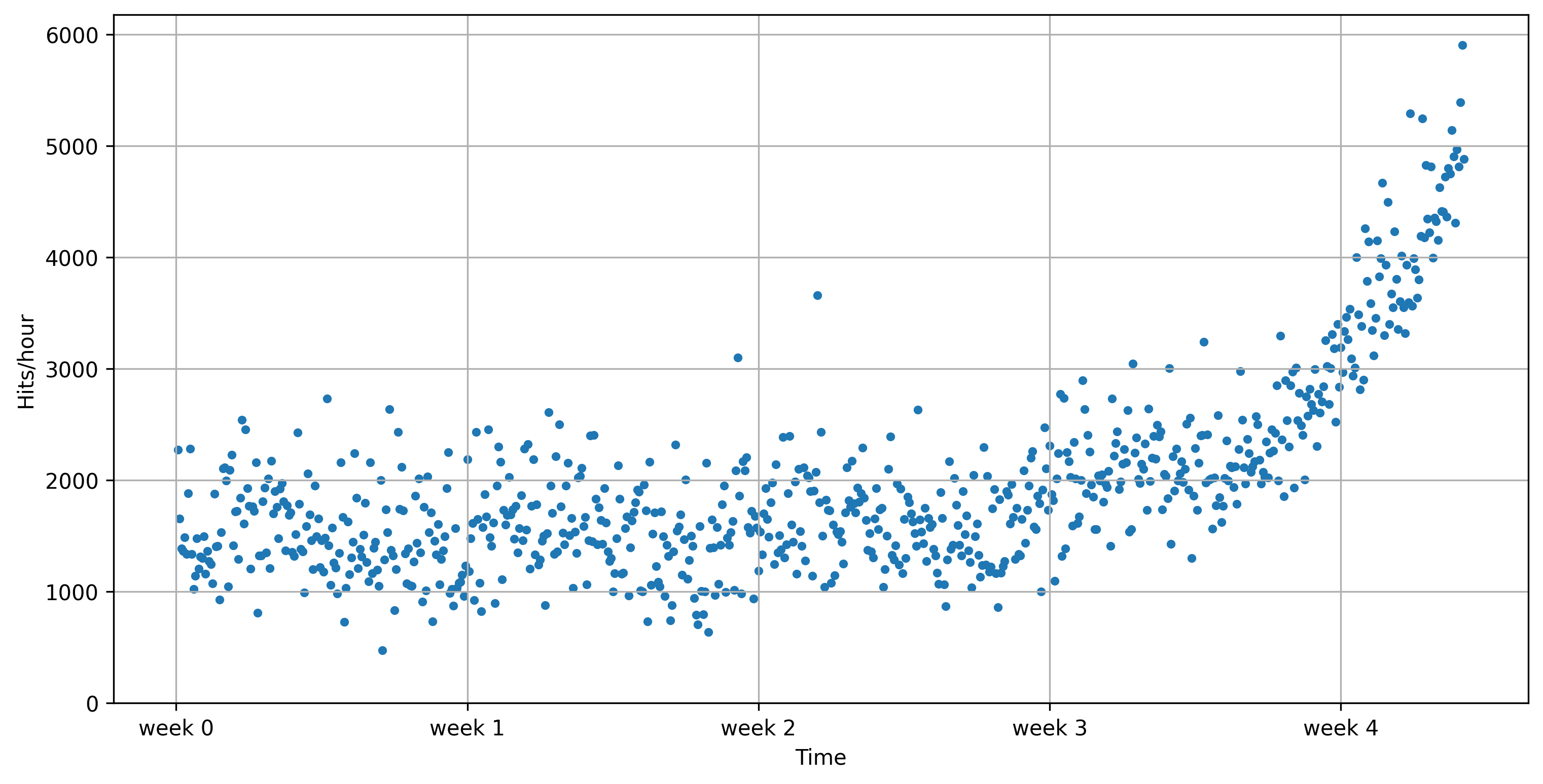
Example: Modelling web traffic#

We generate some artificial data to mimic web traffic data
- E.g. website visits, tweets with certain hashtag,…
- Weekly rhythm + noise + exponential increase

x, y = gen_web_traffic_data()
plot_web_traffic(x, y)

../_images/e490a46f445cb82d369c5e78b7db2943fe5f93d2d56926e66e4367214378207e.png

Use numpy to fit some polynomial lines#

polyfit fits a polynomial of degree d
poly1d evaluates the function using the learned coefficients
Plot with matplotlib

f2 = np.poly1d(np.polyfit(x, y, 2))
f10 = np.poly1d(np.polyfit(x, y, 10))
f50 = np.poly1d(np.polyfit(x, y, 50))

mx = np.linspace(0, x[-1], 1000)
plt.plot(mx, f2(mx))

f2 = np.poly1d(np.polyfit(x, y, 2))
f10 = np.poly1d(np.polyfit(x, y, 10))
f50 = np.poly1d(np.polyfit(x, y, 50))
plot_web_traffic(x, y, [f2,f10,f50])

/Users/jvanscho/miniforge3/lib/python3.9/site-packages/IPython/core/interactiveshell.py:3457: RankWarning: Polyfit may be poorly conditioned
  exec(code_obj, self.user_global_ns, self.user_ns)

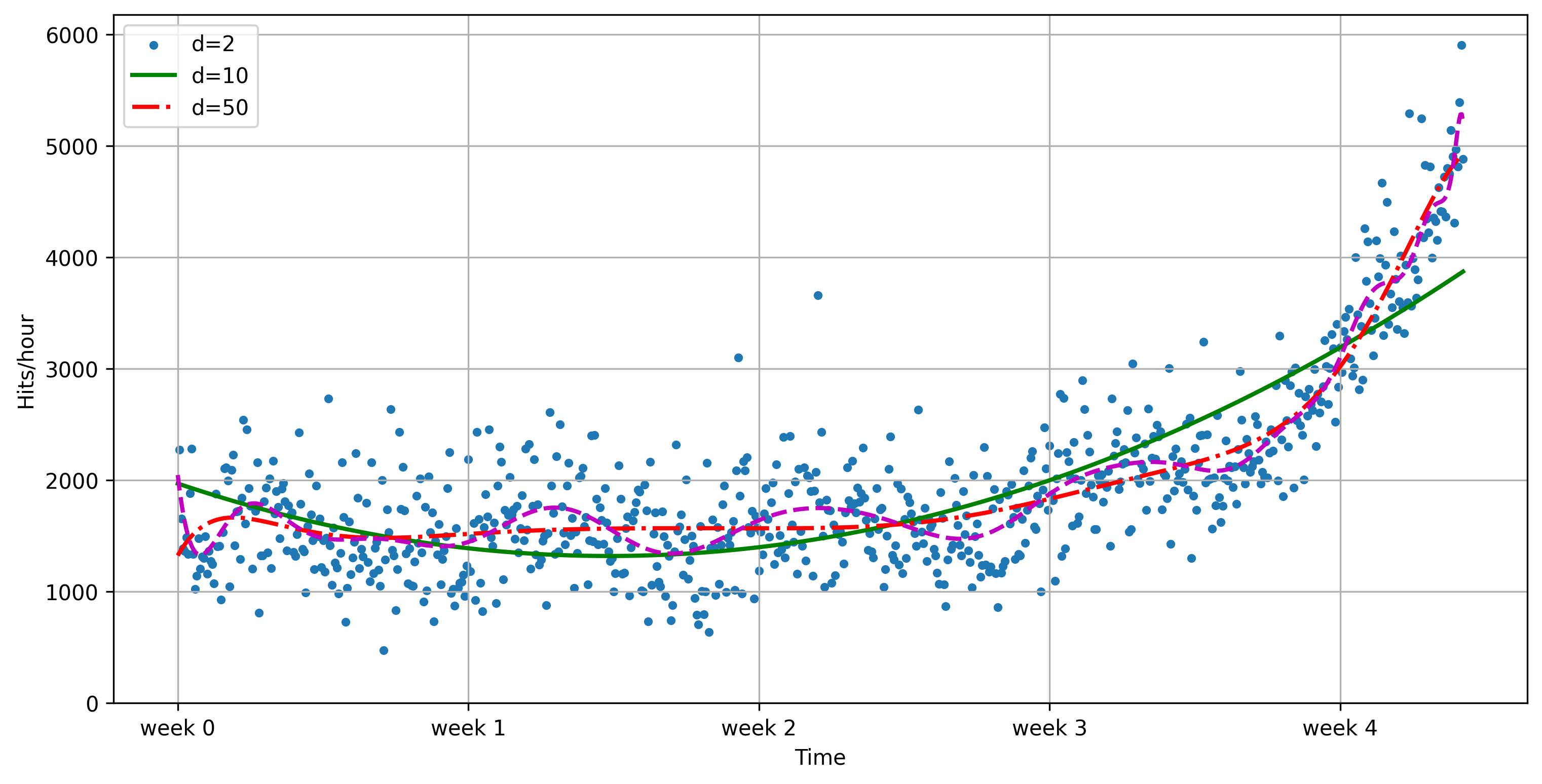
../_images/98e808b40f525b30b3d8da1725a5cb7ccc098fec391bd5937fba97024992b40f.png

Evaluate#

Using root mean squared error: \(\sqrt{\sum_i (f(x_i) - y_i)^2}\)
The degree of the polynomial needs to be tuned to the data
Predictions don’t look great. We need more sophisticated methods.

import ipywidgets as widgets
from ipywidgets import interact, interact_manual

mx=np.linspace(0, 6 * 7 * 24, 100)

def error(f, x, y):
    return np.sqrt(np.sum((f(x)-y)**2))

@interact
def play_with_degree(degree=(1,30,2)):
    f = np.poly1d(np.polyfit(x, y, degree))
    plot_web_traffic(x, y, [f], mx=mx, ymax=10000)
    print("Training error for d=%i: %f" % (f.order, error(f, x, y)))

scikit-learn#

One of the most prominent Python libraries for machine learning:

Contains many state-of-the-art machine learning algorithms
Builds on numpy (fast), implements advanced techniques
Wide range of evaluation measures and techniques
Offers comprehensive documentation about each algorithm
Widely used, and a wealth of tutorials and code snippets are available
Works well with numpy, scipy, pandas, matplotlib,…

Note: We’ll repeat most of the material below in the lectures and labs on model selection and data preprocessing, but it’s still very useful to study it beforehand.

Algorithms#

See the Reference

Supervised learning:

Linear models (Ridge, Lasso, Elastic Net, …)
Support Vector Machines
Tree-based methods (Classification/Regression Trees, Random Forests,…)
Nearest neighbors
Neural networks
Gaussian Processes
Feature selection

Unsupervised learning:

Clustering (KMeans, …)
Matrix Decomposition (PCA, …)
Manifold Learning (Embeddings)
Density estimation
Outlier detection

Model selection and evaluation:

Cross-validation
Grid-search
Lots of metrics

Data import#

Multiple options:

A few toy datasets are included in sklearn.datasets
Import 1000s of datasets via sklearn.datasets.fetch_openml
You can import data files (CSV) with pandas or numpy

from sklearn.datasets import load_iris, fetch_openml
iris_data = load_iris()
dating_data = fetch_openml(name="SpeedDating")

from sklearn.datasets import load_iris, fetch_openml
iris_data = load_iris()
dating_data = fetch_openml("SpeedDating", version=1)

These will return a Bunch object (similar to a dict)

print("Keys of iris_dataset: {}".format(iris_dataset.keys()))
print(iris_dataset['DESCR'][:193] + "\n...")

print("Keys of iris_dataset: {}".format(iris_data.keys()))
print(iris_data['DESCR'][:193] + "\n...")

Keys of iris_dataset: dict_keys(['data', 'target', 'frame', 'target_names', 'DESCR', 'feature_names', 'filename', 'data_module'])
.. _iris_dataset:

Iris plants dataset
--------------------

**Data Set Characteristics:**

    :Number of Instances: 150 (50 in each of three classes)
    :Number of Attributes: 4 numeric, pre
...

Targets (classes) and features are lists of strings
Data and target values are always numeric (ndarrays)

print("Targets: {}".format(iris_data['target_names']))
print("Features: {}".format(iris_data['feature_names']))
print("Shape of data: {}".format(iris_data['data'].shape))
print("First 5 rows:\n{}".format(iris_data['data'][:5]))
print("Targets:\n{}".format(iris_data['target']))

print("Targets: {}".format(iris_data['target_names']))
print("Features: {}".format(iris_data['feature_names']))
print("Shape of data: {}".format(iris_data['data'].shape))
print("First 5 rows:\n{}".format(iris_data['data'][:5]))
print("Targets:\n{}".format(iris_data['target']))

Targets: ['setosa' 'versicolor' 'virginica']
Features: ['sepal length (cm)', 'sepal width (cm)', 'petal length (cm)', 'petal width (cm)']
Shape of data: (150, 4)
First 5 rows:
[[5.1 3.5 1.4 0.2]
 [4.9 3.  1.4 0.2]
 [4.7 3.2 1.3 0.2]
 [4.6 3.1 1.5 0.2]
 [5.  3.6 1.4 0.2]]
Targets:
[0 0 0 0 0 0 0 0 0 0 0 0 0 0 0 0 0 0 0 0 0 0 0 0 0 0 0 0 0 0 0 0 0 0 0 0 0
 0 0 0 0 0 0 0 0 0 0 0 0 0 1 1 1 1 1 1 1 1 1 1 1 1 1 1 1 1 1 1 1 1 1 1 1 1
 1 1 1 1 1 1 1 1 1 1 1 1 1 1 1 1 1 1 1 1 1 1 1 1 1 1 2 2 2 2 2 2 2 2 2 2 2
 2 2 2 2 2 2 2 2 2 2 2 2 2 2 2 2 2 2 2 2 2 2 2 2 2 2 2 2 2 2 2 2 2 2 2 2 2
 2 2]

Building models#

All scikitlearn estimators follow the same interface

class SupervisedEstimator(...):
    def __init__(self, hyperparam, ...):

    def fit(self, X, y):   # Fit/model the training data
        ...                # given data X and targets y
        return self
     
    def predict(self, X):  # Make predictions
        ...                # on unseen data X  
        return y_pred
    
    def score(self, X, y): # Predict and compare to true
        ...                # labels y                
        return score

Training and testing data#

To evaluate our classifier, we need to test it on unseen data.
train_test_split: splits data randomly in 75% training and 25% test data.

X_train, X_test, y_train, y_test = train_test_split(
    iris_data['data'], iris_data['target'], random_state=0)

from sklearn.model_selection import train_test_split
X_train, X_test, y_train, y_test = train_test_split(
    iris_data['data'], iris_data['target'], 
    random_state=0)
print("X_train shape: {}".format(X_train.shape))
print("y_train shape: {}".format(y_train.shape))
print("X_test shape: {}".format(X_test.shape))
print("y_test shape: {}".format(y_test.shape))

X_train shape: (112, 4)
y_train shape: (112,)
X_test shape: (38, 4)
y_test shape: (38,)

Fitting a model#

The first model we’ll build is a k-Nearest Neighbor classifier.
kNN is included in sklearn.neighbors, so let’s build our first model

knn = KNeighborsClassifier(n_neighbors=1)
knn.fit(X_train, y_train)

from sklearn.neighbors import KNeighborsClassifier
knn = KNeighborsClassifier(n_neighbors=1)
knn.fit(X_train, y_train)

KNeighborsClassifier(n_neighbors=1)

Making predictions#

Let’s create a new example and ask the kNN model to classify it

X_new = np.array([[5, 2.9, 1, 0.2]])
prediction = knn.predict(X_new)
class_name = iris_data['target_names'][prediction]

X_new = np.array([[5, 2.9, 1, 0.2]])
prediction = knn.predict(X_new)
print("Prediction: {}".format(prediction))
print("Predicted target name: {}".format(
       iris_data['target_names'][prediction]))

Prediction: [0]
Predicted target name: ['setosa']

Evaluating the model#

Feeding all test examples to the model yields all predictions

y_pred = knn.predict(X_test)

y_pred = knn.predict(X_test)
print("Test set predictions:\n {}".format(y_pred))

Test set predictions:
 [2 1 0 2 0 2 0 1 1 1 2 1 1 1 1 0 1 1 0 0 2 1 0 0 2 0 0 1 1 0 2 1 0 2 2 1 0
 2]

The score function computes the percentage of correct predictions

knn.score(X_test, y_test)

print("Score: {:.2f}".format(knn.score(X_test, y_test) ))

Score: 0.97

Cross-validation#

More stable, thorough way to estimate generalization performance
k-fold cross-validation (CV): split (randomized) data into k equal-sized parts, called folds
- First, fold 1 is the test set, and folds 2-5 comprise the training set
- Then, fold 2 is the test set, folds 1,3,4,5 comprise the training set
- Compute k evaluation scores, aggregate afterwards (e.g. take the mean)

Cross-validation in scikit-learn#

cross_val_score function with learner, training data, labels
Returns list of all scores
- Does 3-fold CV by default, can be changed via cv hyperparameter
- Default scoring measures are accuracy (classification) or \(R^2\) (regression)
Even though models are built internally, they are not returned

knn = KNeighborsClassifier(n_neighbors=1)
scores = cross_val_score(knn, iris.data, iris.target, cv=5)
print("Cross-validation scores: {}".format(scores))
print("Average cross-validation score: {:.2f}".format(scores.mean()))
print("Variance in cross-validation score: {:.4f}".format(np.var(scores)))

from sklearn.model_selection import cross_val_score
from sklearn.datasets import load_iris

iris = load_iris()
knn = KNeighborsClassifier(n_neighbors=1)

scores = cross_val_score(knn, iris.data, iris.target)
print("Cross-validation scores: {}".format(scores))
print("Average cross-validation score: {:.2f}".format(scores.mean()))
print("Variance in cross-validation score: {:.4f}".format(np.var(scores)))

Cross-validation scores: [0.96666667 0.96666667 0.93333333 0.93333333 1.        ]
Average cross-validation score: 0.96
Variance in cross-validation score: 0.0006

More variants#

Stratified cross-validation: for inbalanced datasets
Leave-one-out cross-validation: for very small datasets
Shuffle-Split cross-validation: whenever you need to shuffle the data first
Repeated cross-validation: more trustworthy, but more expensive
Cross-validation with groups: Whenever your data contains non-independent datapoints, e.g. data points from the same patient
Bootstrapping: sampling with replacement, for extracting statistical properties

Avoid data leakage#

Simply taking the best performing model based on cross-validation performance yields optimistic results
We’ve already used the test data to evaluate each model!
Hence, we don’t have an independent test set to evaluate these hyperparameter settings
- Information ‘leaks’ from test set into the final model
Solution: Set aside part of the training data to evaluate the hyperparameter settings
- Select best model on validation set
- Rebuild the model on the training+validation set
- Evaluate optimal model on the test set

Pipelines#

Many learning algorithms are greatly affected by how you represent the training data
Examples: Scaling, numeric/categorical values, missing values, feature selection/construction
We typically need chain together different algorithms
- Many preprocessing steps
- Possibly many models
This is called a pipeline (or workflow)
The best way to represent data depends not only on the semantics of the data, but also on the kind of model you are using.

Example: Speed dating data#

Data collected from speed dating events
See https://www.openml.org/d/40536
Could also be collected from dating website or app
Real-world data:
- Different numeric scales
- Missing values
- Likely irrelevant features
- Different types: Numeric, categorical,…
- Input errors (e.g. ‘lawyer’ vs ‘Lawyer’)

dating_data = fetch_openml("SpeedDating")

dating_data = fetch_openml("SpeedDating", version=1)

Scaling#

When the features have different scales (their values range between very different minimum and maximum values), one feature will overpower the others. Several scaling techniques are available to solve this:

StandardScaler rescales all features to mean=0 and variance=1
- Does not ensure and min/max value
RobustScaler uses the median and quartiles
- Median m: half of the values < m, half > m
- Lower Quartile lq: 1/4 of values < lq
- Upper Quartile uq: 1/4 of values > uq
- Ignores outliers, brings all features to same scale
MinMaxScaler brings all feature values between 0 and 1
Normalizer scales data such that the feature vector has Euclidean length 1
- Projects data to the unit circle
- Used when only the direction/angle of the data matters

Applying scaling transformations#

Lets apply a scaling transformation manually, then use it to train a learning algorithm
First, split the data in training and test set
Next, we fit the preprocessor on the training data
- This computes the necessary transformation parameters
- For MinMaxScaler, these are the min/max values for every feature
After fitting, we can transform the training and test data

scaler = MinMaxScaler()
scaler.fit(X_train)
X_train_scaled = scaler.transform(X_train)
X_test_scaled = scaler.transform(X_test)

Missing value imputation#

Many sci-kit learn algorithms cannot handle missing value
Imputer replaces specific values
- missing_values (default ‘NaN’) placeholder for the missing value
- strategy:
  - mean, replace using the mean along the axis
  - median, replace using the median along the axis
  - most_frequent, replace using the most frequent value
Many more advanced techniques exist, but not yet in scikit-learn
- e.g. low rank approximations (uses matrix factorization)

imp = Imputer(missing_values='NaN', strategy='mean', axis=0)
imp.fit_transform(X1_train)

Feature encoding#

scikit-learn classifiers only handle numeric data. If your features are categorical, you need to encode them first
LabelEncoder simply replaces each value with an integer value
OneHotEncoder converts a feature of \(n\) values to \(n\) binary features
- Provide categories as array or set to ‘auto’

X_enc = OneHotEncoder(categories='auto').fit_transform(X)

ColumnTransformer can apply different transformers to different features
Transformers can be pipelines doing multiple things

numeric_features = ['age', 'pref_o_attractive']
numeric_transformer = Pipeline(steps=[
    ('imputer', SimpleImputer(strategy='median')),
    ('scaler', StandardScaler())])

categorical_features = ['gender', 'd_d_age', 'field']
categorical_transformer = Pipeline(steps=[
    ('imputer', SimpleImputer(strategy='constant', fill_value='missing')),
    ('onehot', OneHotEncoder(handle_unknown='ignore'))])

preprocessor = ColumnTransformer(
    transformers=[
        ('num', numeric_transformer, numeric_features),
        ('cat', categorical_transformer, categorical_features)])

Building Pipelines#

In scikit-learn, a pipeline combines multiple processing steps in a single estimator
All but the last step should be transformer (have a transform method)
- The last step can be a transformer too (e.g. Scaler+PCA)
It has a fit, predict, and score method, just like any other learning algorithm
Pipelines are built as a list of steps, which are (name, algorithm) tuples
- The name can be anything you want, but can’t contain '__'
- We use '__' to refer to the hyperparameters, e.g. svm__C
Let’s build, train, and score a MinMaxScaler + LinearSVC pipeline:

pipe = Pipeline([("scaler", MinMaxScaler()), ("svm", LinearSVC())])
pipe.fit(X_train, y_train).score(X_test, y_test)

from sklearn.pipeline import Pipeline
from sklearn.preprocessing import MinMaxScaler
from sklearn.svm import LinearSVC
from sklearn.datasets import load_breast_cancer

cancer = load_breast_cancer()

pipe = Pipeline([("scaler", MinMaxScaler()), ("svm", LinearSVC())])

X_train, X_test, y_train, y_test = train_test_split(cancer.data, cancer.target,
                                                    random_state=1)
pipe.fit(X_train, y_train)
print("Test score: {:.2f}".format(pipe.score(X_test, y_test)))

Test score: 0.97

Now with cross-validation:

scores = cross_val_score(pipe, cancer.data, cancer.target)

from sklearn.model_selection import cross_val_score
scores = cross_val_score(pipe, cancer.data, cancer.target)
print("Cross-validation scores: {}".format(scores))
print("Average cross-validation score: {:.2f}".format(scores.mean()))

Cross-validation scores: [0.98245614 0.97368421 0.96491228 0.96491228 0.99115044]
Average cross-validation score: 0.98

We can retrieve the trained SVM by querying the right step indices

pipe.steps[1][1]

pipe.fit(X_train, y_train)
print("SVM component: {}".format(pipe.steps[1][1]))

SVM component: LinearSVC()

Or we can use the named_steps dictionary

pipe.named_steps['svm']

print("SVM component: {}".format(pipe.named_steps['svm']))

SVM component: LinearSVC()

When you don’t need specific names for specific steps, you can use make_pipeline
- Assigns names to steps automatically

pipe_short = make_pipeline(MinMaxScaler(), LinearSVC(C=100))
print("Pipeline steps:\n{}".format(pipe_short.steps))

from sklearn.pipeline import make_pipeline
# abbreviated syntax
pipe_short = make_pipeline(MinMaxScaler(), LinearSVC(C=100))
print("Pipeline steps:\n{}".format(pipe_short.steps))

Pipeline steps:
[('minmaxscaler', MinMaxScaler()), ('linearsvc', LinearSVC(C=100))]

Model selection and Hyperparameter tuning#

There are many algorithms to choose from
Most algorithms have parameters (hyperparameters) that control model complexity
Now that we know how to evaluate models, we can improve them selecting by tuning algorithms for your data

We can basically use any optimization technique to optimize hyperparameters:

Grid search
Random search

More advanced techniques:

Local search
Racing algorithms
Bayesian optimization
Multi-armed bandits
Genetic algorithms

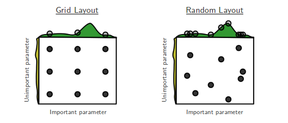
Grid vs Random Search

Grid Search#

For each hyperparameter, create a list of interesting/possible values
- E.g. For kNN: k in [1,3,5,7,9,11,33,55,77,99]
- E.g. For SVM: C and gamma in [\(10^{-10}\)..\(10^{10}\)]
Evaluate all possible combinations of hyperparameter values
- E.g. using cross-validation
Split the training data into a training and validation set
Select the hyperparameter values yielding the best results on the validation set

Grid search in scikit-learn#

Create a parameter grid as a dictionary
- Keys are parameter names
- Values are lists of hyperparameter values

param_grid = {'C': [0.001, 0.01, 0.1, 1, 10, 100],
              'gamma': [0.001, 0.01, 0.1, 1, 10, 100]}
print("Parameter grid:\n{}".format(param_grid))

param_grid = {'C': [0.001, 0.01, 0.1, 1, 10, 100],
              'gamma': [0.001, 0.01, 0.1, 1, 10, 100]}
print("Parameter grid:\n{}".format(param_grid))

Parameter grid:
{'C': [0.001, 0.01, 0.1, 1, 10, 100], 'gamma': [0.001, 0.01, 0.1, 1, 10, 100]}

GridSearchCV: like a classifier that uses CV to automatically optimize its hyperparameters internally
- Input: (untrained) model, parameter grid, CV procedure
- Output: optimized model on given training data
- Should only have access to training data

grid_search = GridSearchCV(SVC(), param_grid, cv=5)
grid_search.fit(X_train, y_train)

from sklearn.model_selection import GridSearchCV 
from sklearn.svm import SVC
grid_search = GridSearchCV(SVC(), param_grid, cv=5)
X_train, X_test, y_train, y_test = train_test_split(
        iris.data, iris.target, random_state=0)
grid_search.fit(X_train, y_train)

GridSearchCV(cv=5, estimator=SVC(),
             param_grid={'C': [0.001, 0.01, 0.1, 1, 10, 100],
                         'gamma': [0.001, 0.01, 0.1, 1, 10, 100]})

The optimized test score and hyperparameters can easily be retrieved:

grid_search.score(X_test, y_test)
grid_search.best_params_
grid_search.best_score_
grid_search.best_estimator_

print("Test set score: {:.2f}".format(grid_search.score(X_test, y_test)))
print("Best parameters: {}".format(grid_search.best_params_))
print("Best cross-validation score: {:.2f}".format(grid_search.best_score_))
print("Best estimator:\n{}".format(grid_search.best_estimator_))

Test set score: 0.97
Best parameters: {'C': 10, 'gamma': 0.1}
Best cross-validation score: 0.97
Best estimator:
SVC(C=10, gamma=0.1)

Nested cross-validation#

Note that we are still using a single split to create the outer test set
We can also use cross-validation here
Nested cross-validation:
- Outer loop: split data in training and test sets
- Inner loop: run grid search, splitting the training data into train and validation sets
Result is a just a list of scores
- There will be multiple optimized models and hyperparameter settings (not returned)
To apply on future data, we need to train GridSearchCV on all data again

scores = cross_val_score(GridSearchCV(SVC(), param_grid, cv=5),
                         iris.data, iris.target, cv=5)

scores = cross_val_score(GridSearchCV(SVC(), param_grid, cv=5),
                         iris.data, iris.target, cv=5)
print("Cross-validation scores: ", scores)
print("Mean cross-validation score: ", scores.mean())

Cross-validation scores:  [0.96666667 1.         0.96666667 0.96666667 1.        ]
Mean cross-validation score:  0.9800000000000001

Random Search#

Grid Search has a few downsides:
- Optimizing many hyperparameters creates a combinatorial explosion
- You have to predefine a grid, hence you may jump over optimal values
Random Search:
- Picks n_iter random parameter values
- Scales better, you control the number of iterations
- Often works better in practice, too
  - not all hyperparameters interact strongly
  - you don’t need to explore all combinations

Executing random search in scikit-learn:
- RandomizedSearchCV works like GridSearchCV
- Has n_iter parameter for the number of iterations
- Search grid can use distributions instead of fixed lists

param_grid = {'C': expon(scale=100), 
              'gamma': expon(scale=.1)}
random_search = RandomizedSearchCV(SVC(), param_distributions=param_grid,
                                   n_iter=20)
random_search.fit(X_train, y_train)
random_search.best_estimator_

from sklearn.model_selection import RandomizedSearchCV
from scipy.stats import expon

param_grid = {'C': expon(scale=100), 
              'gamma': expon(scale=.1)}
random_search = RandomizedSearchCV(SVC(), param_distributions=param_grid,
                                   n_iter=20)
X_train, X_test, y_train, y_test = train_test_split(
        iris.data, iris.target, random_state=0)
random_search.fit(X_train, y_train)
random_search.best_estimator_

SVC(C=210.39084256954456, gamma=0.003623016212739808)

Using Pipelines in Grid-searches#

We can use the pipeline as a single estimator in cross_val_score or GridSearchCV
To define a grid, refer to the hyperparameters of the steps
- Step svm, parameter C becomes svm__C

param_grid = {'svm__C': [0.001, 0.01, 0.1, 1, 10, 100],
              'svm__gamma': [0.001, 0.01, 0.1, 1, 10, 100]}
pipe = pipeline.Pipeline([("scaler", MinMaxScaler()), ("svm", SVC(C=100))])
grid = GridSearchCV(pipe, param_grid=param_grid, cv=5)
grid.fit(X_train, y_train)

param_grid = {'svm__C': [0.001, 0.01, 0.1, 1, 10, 100],
              'svm__gamma': [0.001, 0.01, 0.1, 1, 10, 100]}

from sklearn import pipeline
from sklearn.svm import SVC
from sklearn.model_selection import GridSearchCV


pipe = pipeline.Pipeline([("scaler", MinMaxScaler()), ("svm", SVC(C=100))])
grid = GridSearchCV(pipe, param_grid=param_grid, cv=5)
grid.fit(X_train, y_train)
print("Best cross-validation accuracy: {:.2f}".format(grid.best_score_))
print("Test set score: {:.2f}".format(grid.score(X_test, y_test)))
print("Best parameters: {}".format(grid.best_params_))

Best cross-validation accuracy: 0.96
Test set score: 0.97
Best parameters: {'svm__C': 1, 'svm__gamma': 10}

Automated Machine Learning#

Optimizes both the pipeline and all hyperparameters
E.g. auto-sklearn
- Drop-in sklearn classifier
- Also optimizes pipelines (e.g. feature selection)
- Uses OpenML to find good models on similar datasets
- Lacks Windows support

automl = autosklearn.classification.AutoSklearnClassifier(
    time_left_for_this_task=60, # sec., for entire process
    per_run_time_limit=15, # sec., for each model
    ml_memory_limit=1024, # MB, memory limit
)
automl.fit(X_train, y_train)