Lecture 8. Transformers

Lecture 8. Transformers#

Maybe attention is all you need

Joaquin Vanschoren

# Auto-setup when running on Google Colab
import os
if 'google.colab' in str(get_ipython()) and not os.path.exists('/content/master'):
    !git clone -q https://github.com/ML-course/master.git /content/master
    !pip --quiet install -r /content/master/requirements_colab.txt
    %cd master/notebooks

# Global imports and settings
%matplotlib inline
from preamble import *
interactive = True # Set to True for interactive plots 
if interactive:
    fig_scale = 0.5
    plt.rcParams.update(print_config)
else: # For printing
    fig_scale = 0.4
    plt.rcParams.update(print_config)
    
HTML('''<style>.rise-enabled .reveal pre {font-size=75%} </style>''')

Overview#

Basics: word embeddings
- Word2Vec, FastText, GloVe
Sequence-to-sequence and autoregressive models
Self-attention and transformer models
Vision Transformers

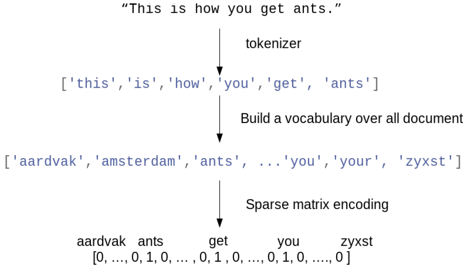
Bag of word representation#

First, build a vocabulary of all occuring words. Maps every word to an index.
Represent each document as an $N$ dimensional vector (top-$N$ most frequent words)
- One-hot (sparse) encoding: 1 if the word occurs in the document
Destroys the order of the words in the text (hence, a ‘bag’ of words)

Text preprocessing pipelines#

Tokenization: how to you split text into words / tokens?
Stemming: naive reduction to word stems. E.g. ‘the meeting’ to ‘the meet’
Lemmatization: NLP-based reduction, e.g. distinguishes between nouns and verbs
Discard stop words (‘the’, ‘an’,…)
Only use $N$ (e.g. 10000) most frequent words, or a hash function
n-grams: Use combinations of $n$ adjacent words next to individual words
- e.g. 2-grams: “awesome movie”, “movie with”, “with creative”, …
Character n-grams: combinations of $n$ adjacent letters: ‘awe’, ‘wes’, ‘eso’,…
Subword tokenizers: graceful splits “unbelievability” -> un, believ, abil, ity
Useful libraries: nltk, spaCy, gensim, HuggingFace tokenizers,…

Scaling#

Only for classical models, LLMs use subword tokenizers and dense tokens from embedding layers (see later)
L2 Normalization (vector norm): sum of squares of all word values equals 1
- Normalized Euclidean distance is equivalent to cosine distance
- Works better for distance-based models (e.g. kNN, SVM,…) $$ t_i = \frac{t_i}{\| t\|_2 }$$
Term Frequency - Inverted Document Frequency (TF-IDF)
- Scales value of words by how frequently they occur across all $N$ documents
- Words that only occur in few documents get higher weight, and vice versa

\[ t_i = t_i \cdot log(\frac{N}{|\{d \in D : t_i \in d\}|})\]

Neural networks on bag of words#

We can build neural networks on bag-of-word vectors
- Do a one-hot-encoding with 10000 most frequent words
- Simple model with 2 dense layers, ReLU activation, dropout

self.model = nn.Sequential(
    nn.Linear(10000, 16),
    nn.ReLU(),
    nn.Dropout(0.5),
    nn.Linear(16, 16),
    nn.ReLU(),
    nn.Dropout(0.5),
    nn.Linear(16, 1)
)

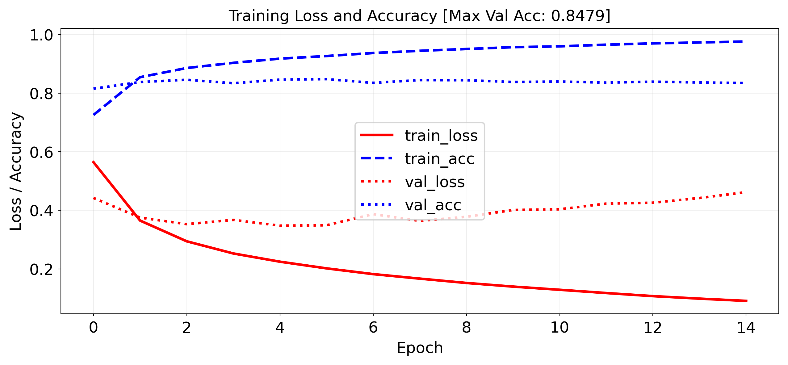
Evaluation#

IMDB dataset of movie reviews (label is ‘positive’ or ‘negative’)
Take a validation set of 10,000 samples from the training set
Works prety well (88% Acc), but overfits easily

import torch
from torch.utils.data import DataLoader, Dataset, random_split
from collections import Counter
import torch.nn as nn
import torch.nn.functional as F
import pytorch_lightning as pl
from keras.datasets import imdb
from IPython.display import clear_output

# Load data with top 10,000 words
(train_data, train_labels), (test_data, test_labels) = imdb.load_data(num_words=10000)

# Vectorize sequences into one-hot encoded vectors
def vectorize_sequences(sequences, dimension=10000):
    results = np.zeros((len(sequences), dimension), dtype=np.float32)
    for i, sequence in enumerate(sequences):
        results[i, sequence] = 1.0
    return results

# One-hot encode
x_train = vectorize_sequences(train_data)
x_test = vectorize_sequences(test_data)
y_train = np.asarray(train_labels).astype('float32')
y_test = np.asarray(test_labels).astype('float32')

class IMDBVectorizedDataset(Dataset):
    def __init__(self, features, labels):
        self.x = torch.tensor(features, dtype=torch.float32)
        self.y = torch.tensor(labels, dtype=torch.float32)

    def __len__(self):
        return len(self.x)

    def __getitem__(self, idx):
        return self.x[idx], self.y[idx]
    
# Validation split like in Keras: first 10k for val
x_val, x_partial_train = x_train[:10000], x_train[10000:]
y_val, y_partial_train = y_train[:10000], y_train[10000:]

train_dataset = IMDBVectorizedDataset(x_partial_train, y_partial_train)
val_dataset = IMDBVectorizedDataset(x_val, y_val)
test_dataset = IMDBVectorizedDataset(x_test, y_test)

train_loader = DataLoader(train_dataset, batch_size=512, shuffle=True)
val_loader = DataLoader(val_dataset, batch_size=512)
test_loader = DataLoader(test_dataset, batch_size=512)

class LivePlotCallback(pl.Callback):
    def __init__(self):
        self.train_losses = []
        self.train_accs = []
        self.val_losses = []
        self.val_accs = []
        self.max_acc = 0

    def on_train_epoch_end(self, trainer, pl_module):
        metrics = trainer.callback_metrics

        train_loss = metrics.get("train_loss")
        train_acc = metrics.get("train_acc")
        val_loss = metrics.get("val_loss")
        val_acc = metrics.get("val_acc")

        if all(v is not None for v in [train_loss, train_acc, val_loss, val_acc]):
            self.train_losses.append(train_loss.item())
            self.train_accs.append(train_acc.item())
            self.val_losses.append(val_loss.item())
            self.val_accs.append(val_acc.item())
            self.max_acc = max(self.max_acc, val_acc.item())

            if len(self.train_losses) > 1:
                clear_output(wait=True)
                N = np.arange(0, len(self.train_losses))
                plt.figure(figsize=(10, 4))
                plt.plot(N, self.train_losses, label='train_loss', lw=2, c='r')
                plt.plot(N, self.train_accs, label='train_acc', lw=2, c='b')
                plt.plot(N, self.val_losses, label='val_loss', lw=2, linestyle=":", c='r')
                plt.plot(N, self.val_accs, label='val_acc', lw=2, linestyle=":", c='b')
                plt.title(f"Training Loss and Accuracy [Max Val Acc: {self.max_acc:.4f}]", fontsize=12)
                plt.xlabel("Epoch", fontsize=12)
                plt.ylabel("Loss / Accuracy", fontsize=12)
                plt.tick_params(axis='both', labelsize=12)
                plt.legend(fontsize=12)
                plt.grid(True)
                plt.show()
            
class IMDBClassifier(pl.LightningModule):
    def __init__(self):
        super().__init__()
        self.fc1 = nn.Linear(10000, 16)
        self.dropout1 = nn.Dropout(0.5)
        self.fc2 = nn.Linear(16, 16)
        self.dropout2 = nn.Dropout(0.5)
        self.fc3 = nn.Linear(16, 1)

    def forward(self, x):
        x = F.relu(self.fc1(x))
        x = self.dropout1(x)
        x = F.relu(self.fc2(x))
        x = self.dropout2(x)
        x = torch.sigmoid(self.fc3(x))
        return x.squeeze()

    def training_step(self, batch, batch_idx):
        x, y = batch
        y_hat = self(x)
        loss = F.binary_cross_entropy(y_hat, y)
        acc = ((y_hat > 0.5) == y.bool()).float().mean()
        self.log("train_loss", loss, on_step=False, on_epoch=True, prog_bar=True)
        self.log("train_acc", acc, on_step=False, on_epoch=True, prog_bar=True)
        return loss

    def validation_step(self, batch, batch_idx):
        x, y = batch
        y_hat = self(x)
        val_loss = F.binary_cross_entropy(y_hat, y)
        val_acc = ((y_hat > 0.5) == y.bool()).float().mean()
        self.log("val_loss", val_loss, on_epoch=True, prog_bar=True)
        self.log("val_acc", val_acc, on_epoch=True, prog_bar=True)

    def configure_optimizers(self):
        return torch.optim.RMSprop(self.parameters())
    
model = IMDBClassifier()
trainer = pl.Trainer(max_epochs=15, callbacks=[LivePlotCallback()], logger=False, enable_checkpointing=False)
trainer.fit(model, train_dataloaders=train_loader, val_dataloaders=val_loader)

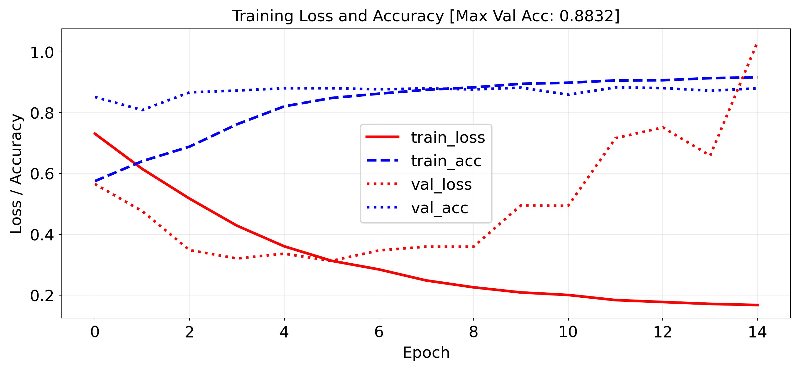
../_images/366036042588febc99e41780fc5fcb755ebcb55af43d3f4118afa4173e137ad9.png

`Trainer.fit` stopped: `max_epochs=15` reached.

Predictions#

Let’s look at a few predictions. Why is the last one so negative?

# 1. Get the trained model into eval mode
model.eval()

# 2. Disable gradient tracking
with torch.no_grad():
    # Convert entire test set to a tensor if not already
    x_test_tensor = torch.tensor(x_test, dtype=torch.float32)

    # Get predictions
    predictions = model(x_test_tensor).numpy()

# Get word index from Keras
word_index = imdb.get_word_index()
word_index = {k: (v + 3) for k, v in word_index.items()}
reverse_word_index = {value: key for key, value in word_index.items()}

# Add special tokens
reverse_word_index[0] = '[PAD]'
reverse_word_index[1] = '[START]'
reverse_word_index[2] = '[UNK]'
reverse_word_index[3] = '[UNUSED]'

def encode_review(text, word_index, num_words=10000):
    # Basic preprocessing
    words = text.lower().split()
    encoded = [1]  # 1 is the index for [START]

    for word in words:
        index = word_index.get(word, 2)  # 2 is [UNK]
        if index < num_words:
            encoded.append(index)
    return encoded

# Function to decode a review
def decode_review(encoded_review):
    return ' '.join([reverse_word_index.get(i, '?') for i in encoded_review])

print("Review 0:\n", decode_review(test_data[0]))
print("Predicted positiveness:", predictions[0])

print("\nReview 16:\n", decode_review(test_data[16]))
print("Predicted positiveness:", predictions[16])

# New sentence
sentence = '[START] this movie was not too terrible'
encoded = encode_review(sentence, word_index)
vectorized = vectorize_sequences([encoded])  # Note: wrap in list to get shape (1, 10000)
model.eval()
with torch.no_grad():
    input_tensor = torch.tensor(vectorized, dtype=torch.float32)
    prediction = model(input_tensor).item()

print("\nReview X:\n",sentence)
print(f"Predicted positiveness: {prediction:.4f}")

Review 0:
 [START] please give this one a miss br br [UNK] [UNK] and the rest of the cast rendered terrible performances the show is flat flat flat br br i don't know how michael madison could have allowed this one on his plate he almost seemed to know this wasn't going to work out and his performance was quite [UNK] so all you madison fans give this a miss
Predicted positiveness: 0.0010664713

Review 16:
 [START] from 1996 first i watched this movie i feel never reach the end of my satisfaction i feel that i want to watch more and more until now my god i don't believe it was ten years ago and i can believe that i almost remember every word of the dialogues i love this movie and i love this novel absolutely perfection i love willem [UNK] he has a strange voice to spell the words black night and i always say it for many times never being bored i love the music of it's so much made me come into another world deep in my heart anyone can feel what i feel and anyone could make the movie like this i don't believe so thanks thanks
Predicted positiveness: 0.99484247

Review X:
 [START] this movie was not too terrible
Predicted positiveness: 0.0198

Word Embeddings#

A word embedding is a numeric vector representation of a word
- Can be manual or learned from an existing representation (e.g. one-hot)

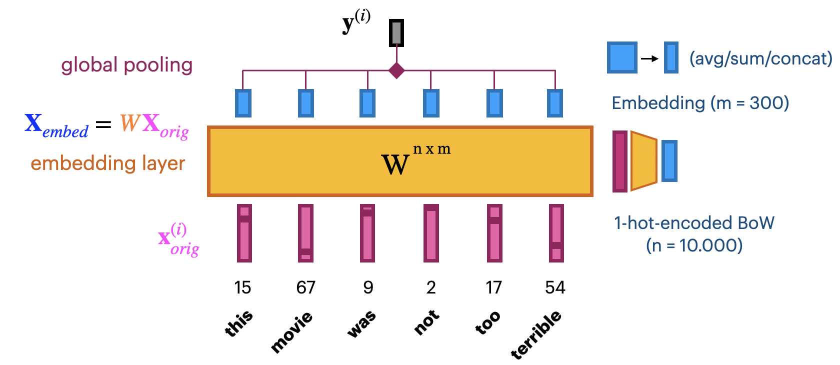
Learning embeddings from scratch#

Input layer uses fixed length documents (with 0-padding).
Add an embedding layer to learn the embedding
- Create $n$-dimensional one-hot encoding.
- To learn an $m$-dimensional embedding, use $m$ hidden nodes. Weight matrix $W^{n x m}$
- Linear activation function: $\mathbf{X}_{embed} = W \mathbf{X}_{orig}$.
Combine all word embeddings into a document embedding (e.g. global pooling).
Add layers to map word embeddings to the output. Learn embedding weights from data.

Let’s try this:

max_length = 100 # pad documents to a maximum number of words
vocab_size = 10000 # vocabulary size
embedding_length = 20 # embedding length (more would be better)

self.model = nn.Sequential(
    nn.Embedding(vocab_size, embedding_length),
    nn.AdaptiveAvgPool1d(1),  # global average pooling over sequence
    nn.Linear(embedding_length, 1),
)

Training on the IMDB dataset: slightly worse than using bag-of-words?
- Embedding of dim 20 is very small, should be closer to 100 (or 300)
- We don’t have enough data to learn a really good embedding from scratch

import torch
import torch.nn as nn
import torch.nn.functional as F
import pytorch_lightning as pl

class IMDBVectorizedDataset(Dataset):
    def __init__(self, features, labels):
        self.x = torch.tensor(features, dtype=torch.long) # Needs long
        self.y = torch.tensor(labels, dtype=torch.float32)

    def __len__(self):
        return len(self.x)

    def __getitem__(self, idx):
        return self.x[idx], self.y[idx]

class IMDBEmbeddingModel(pl.LightningModule):
    def __init__(self, vocab_size=10000, embedding_length=20, max_length=100):
        super().__init__()
        self.embedding = nn.Embedding(vocab_size, embedding_length)
        self.pooling = nn.AdaptiveAvgPool1d(1)  # GlobalAveragePooling1D equivalent
        self.fc = nn.Linear(embedding_length, 1)

    def forward(self, x):
        # x: (batch, max_length)
        embedded = self.embedding(x)  # (batch, max_length, embedding_length)
        embedded = embedded.permute(0, 2, 1)  # for AdaptiveAvgPool1d → (batch, embed_dim, seq_len)
        pooled = self.pooling(embedded).squeeze(-1)  # → (batch, embed_dim)
        output = torch.sigmoid(self.fc(pooled))  # → (batch, 1)
        return output.squeeze()

    def training_step(self, batch, batch_idx):
        x, y = batch
        y_hat = self(x)
        loss = F.binary_cross_entropy(y_hat, y)
        acc = ((y_hat > 0.5) == y.bool()).float().mean()
        self.log("train_loss", loss, on_step=False, on_epoch=True, prog_bar=True)
        self.log("train_acc", acc, on_step=False, on_epoch=True, prog_bar=True)
        return loss

    def validation_step(self, batch, batch_idx):
        x, y = batch
        y_hat = self(x)
        val_loss = F.binary_cross_entropy(y_hat, y)
        val_acc = ((y_hat > 0.5) == y.bool()).float().mean()
        self.log("val_loss", val_loss, on_epoch=True, prog_bar=True)
        self.log("val_acc", val_acc, on_epoch=True, prog_bar=True)

    def configure_optimizers(self):
        return torch.optim.RMSprop(self.parameters())

# Build padded sequences
from keras.preprocessing.sequence import pad_sequences

# Parameters
vocab_size = 10000
max_length = 100

# Load and preprocess
(train_data, train_labels), (test_data, test_labels) = imdb.load_data(num_words=vocab_size)
x_train = pad_sequences(train_data, maxlen=max_length)
x_test = pad_sequences(test_data, maxlen=max_length)

y_train = train_labels
y_test = test_labels

# Split training/validation like in Keras example
x_val, x_partial_train = x_train[:10000], x_train[10000:]
y_val, y_partial_train = y_train[:10000], y_train[10000:]

from torch.utils.data import DataLoader

train_dataset = IMDBVectorizedDataset(x_partial_train, y_partial_train)
val_dataset = IMDBVectorizedDataset(x_val, y_val)
test_dataset = IMDBVectorizedDataset(x_test, y_test)

train_loader = DataLoader(train_dataset, batch_size=512, shuffle=True)
val_loader = DataLoader(val_dataset, batch_size=512)
test_loader = DataLoader(test_dataset, batch_size=512)

model = IMDBEmbeddingModel(vocab_size=vocab_size, embedding_length=20, max_length=max_length)

trainer = pl.Trainer(
    max_epochs=15,
    logger=False,
    enable_checkpointing=False,
    callbacks=[LivePlotCallback()]  # optional
)

trainer.fit(model, train_dataloaders=train_loader, val_dataloaders=val_loader)

../_images/5172594d55ef6df56536d9841668c7d9cc39ec354888e8b9c4986258cccab702.png

`Trainer.fit` stopped: `max_epochs=15` reached.

Pre-trained embeddings#

With more data we can build better embeddings, but we also need more labels
Solution: transfer learning! Learn embedding on auxiliary task that doesn’t require labels
- E.g. given a word, predict the surrounding words.
- Also called self-supervised learning. Supervision is provided by data itself
Freeze embedding weights to produce simple word embeddings, or finetune to a new tasks
Most common approaches:
- Word2Vec: Learn neural embedding for a word based on surrounding words
- FastText: learns embedding for character n-grams
  - Can also produce embeddings for new, unseen words
- GloVe (Global Vector): Count co-occurrences of words in a matrix
  - Use a low-rank approximation to get a latent vector representation

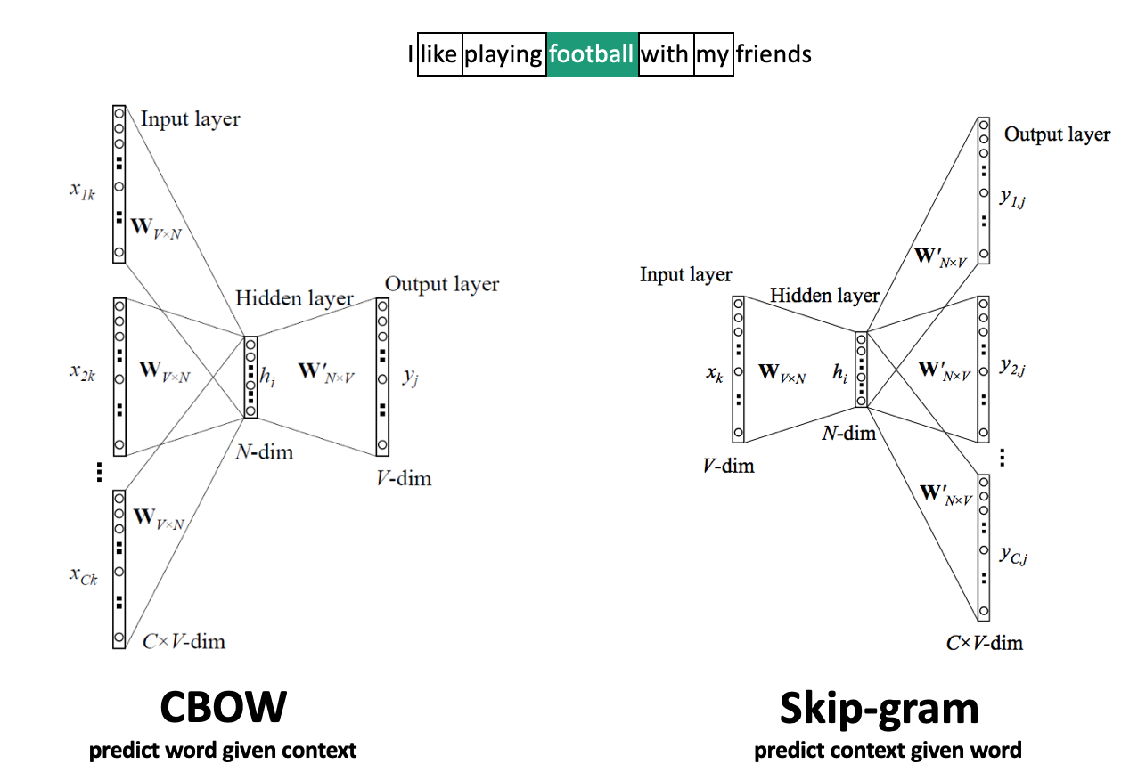
Word2Vec#

Move a window over text to get $C$ context words ($V$-dim one-hot encoded)
Add embedding layer with $N$ linear nodes, global average pooling, and softmax layer(s)
CBOW: predict word given context, use weights of last layer $W^{'}_{NxV}$ as embedding
Skip-Gram: predict context given word, use weights of first layer $W^{T}_{VxN}$ as embedding
- Scales to larger text corpora, learns relationships between words better

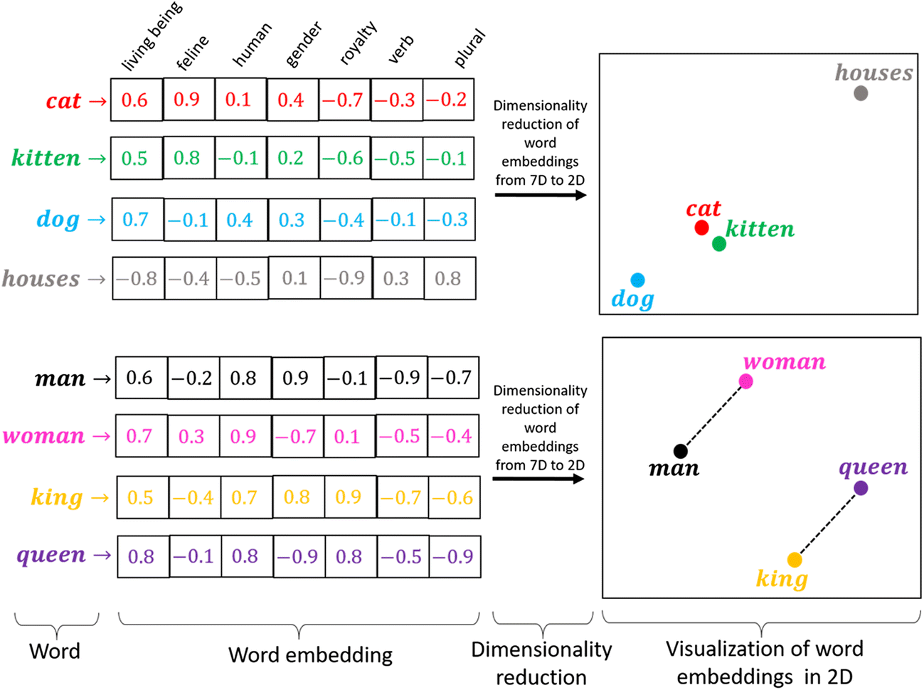
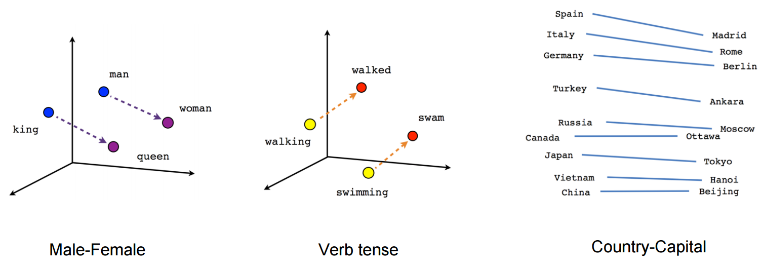
Word2Vec properties#

Word2Vec happens to learn interesting relationships between words
- Simple vector arithmetic can map words to plurals, conjugations, gender analogies,…
- e.g. Gender relationships: $vec_{king} - vec_{man} + vec_{woman} \sim vec_{queen}$
- PCA applied to embeddings shows Country - Capital relationship
Careful: embeddings can capture gender and other biases present in the data.
- Important unsolved problem!

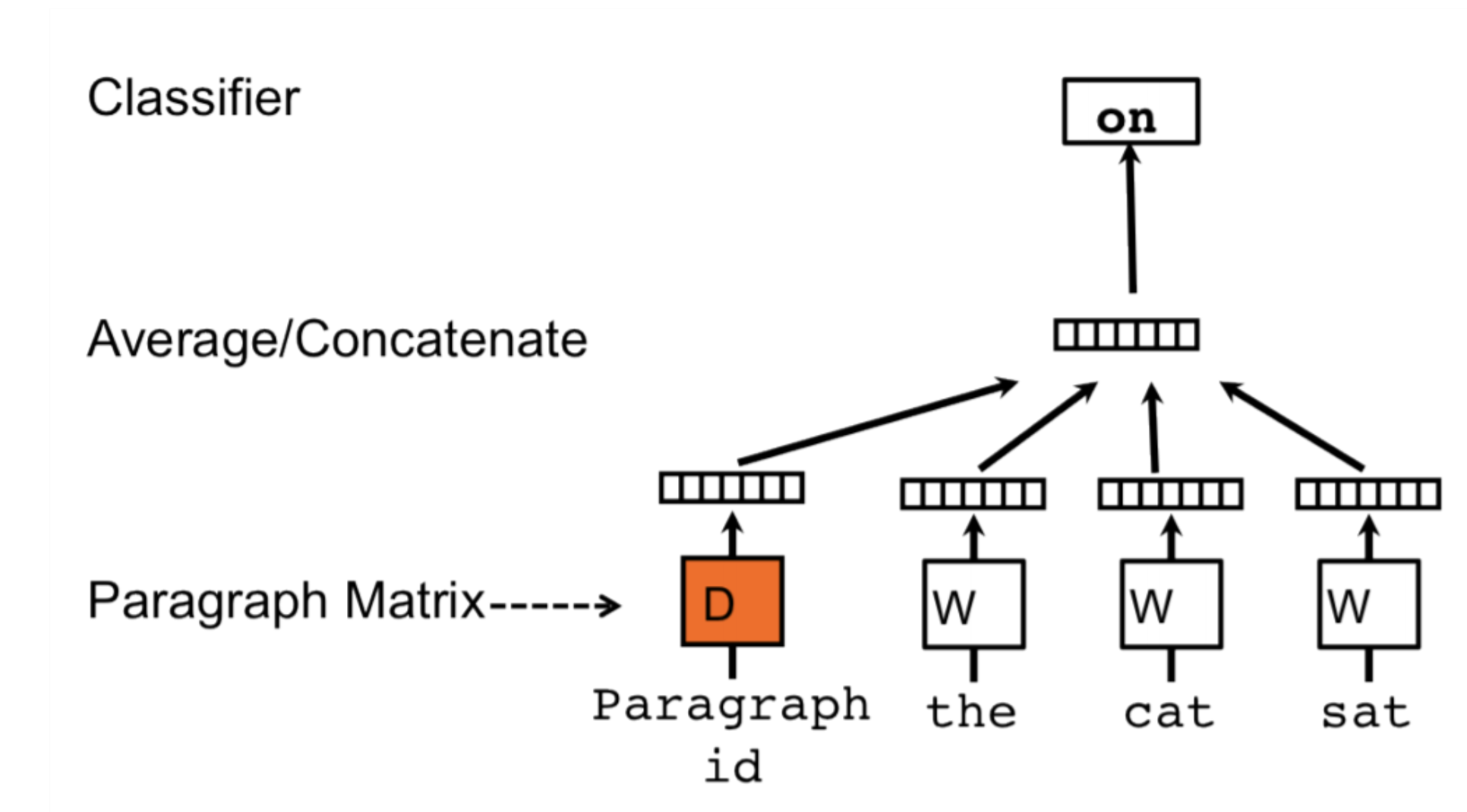
Doc2Vec#

Alternative way to combine word embeddings (instead of global pooling)
Adds a paragraph (or document) embedding: learns how paragraphs (or docs) relate to each other
- Captures document-level semantics: context and meaning of entire document
Can be used to determine semantic similarity between documents.

FastText#

Limitations of Word2Vec:
- Cannot represent new (out-of-vocabulary) words
- Similar words are learned independently: less efficient (no parameter sharing)
  - E.g. ‘meet’ and ‘meeting’
FastText: same model, but uses character n-grams
- Words are represented by all character n-grams of length 3 to 6
  - “football” 3-grams: <fo, foo, oot, otb, tba, bal, all, ll>
- Because there are so many n-grams, they are hashed (dimensionality = bin size)
- Representation of word “football” is sum of its n-gram embeddings
Negative sampling: also trains on random negative examples (out-of-context words)
- Weights are updated so that they are less likely to be predicted

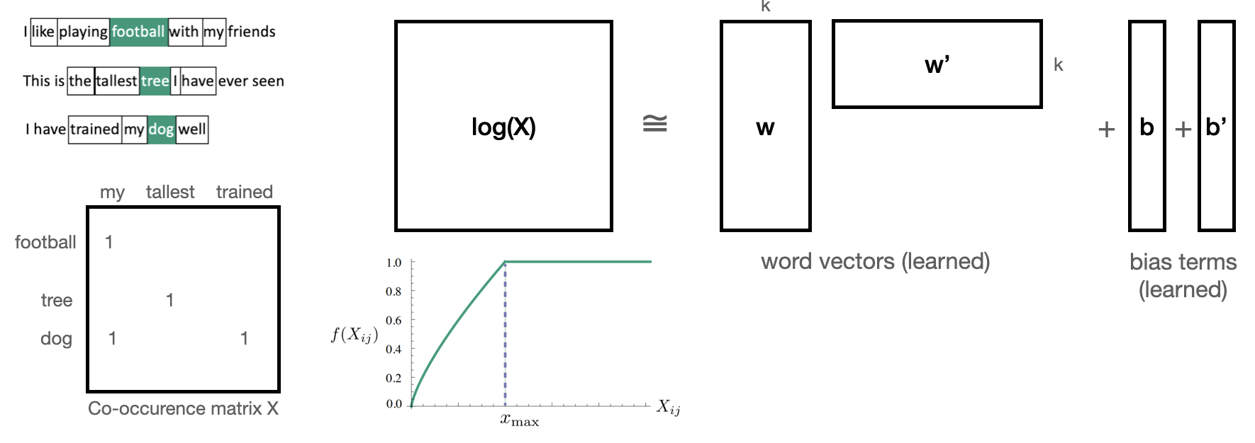
Global Vector model (GloVe)#

Builds a co-occurence matrix $\mathbf{X}$: counts how often 2 words occur in the same context
Learns a k-dimensional embedding $W$ through matrix factorization with rank k
- Actually learns 2 embeddings $W$ and $W'$ (differ in random initialization)
Minimizes loss $\mathcal{L}$, where $b_i$ and $b'_i$ are bias terms and $f$ is a weighting function

\[\mathcal{L} = \sum_{i,j=1}^{V} f(\mathbf{X}_{ij}) (\mathbf{w_i} \mathbf{w'_j} + b_i + b'_j - log(\mathbf{X}_{ij}))^2\]

Let’s try this

Download the GloVe embeddings trained on Wikipedia
We can now get embeddings for 400,000 English words
E.g. ‘queen’ (50 first values of 300-dim embedding)

# To find the original data files, see
# http://nlp.stanford.edu/data/glove.6B.zip
# http://www.cs.cmu.edu/afs/cs.cmu.edu/project/theo-20/www/data/news20.tar.gz

# Build an index so that we can later easily compose the embedding matrix
data_dir = '../data'
embeddings_index = {}
with open(os.path.join(data_dir, 'glove.txt')) as f:
    for line in f:
        word, coefs = line.split(maxsplit=1)
        coefs = np.fromstring(coefs, "f", sep=" ")
        embeddings_index[word] = coefs

print('Found %s word vectors.' % len(embeddings_index))

Found 400000 word vectors.

embeddings_index['queen'][0:50]

array([-0.222,  0.065, -0.086,  0.513,  0.325, -0.129,  0.083,  0.092,
       -0.309, -0.941, -0.089, -0.108,  0.211,  0.701,  0.268, -0.04 ,
        0.174, -0.308, -0.052, -0.175, -0.841,  0.192, -0.138,  0.385,
        0.272, -0.174, -0.466, -0.025,  0.097,  0.301,  0.18 , -0.069,
       -0.205,  0.357, -0.283,  0.281, -0.012,  0.107, -0.244, -0.179,
       -0.132, -0.17 , -0.594,  0.957,  0.204, -0.043,  0.607, -0.069,
        0.523, -0.548], dtype=float32)

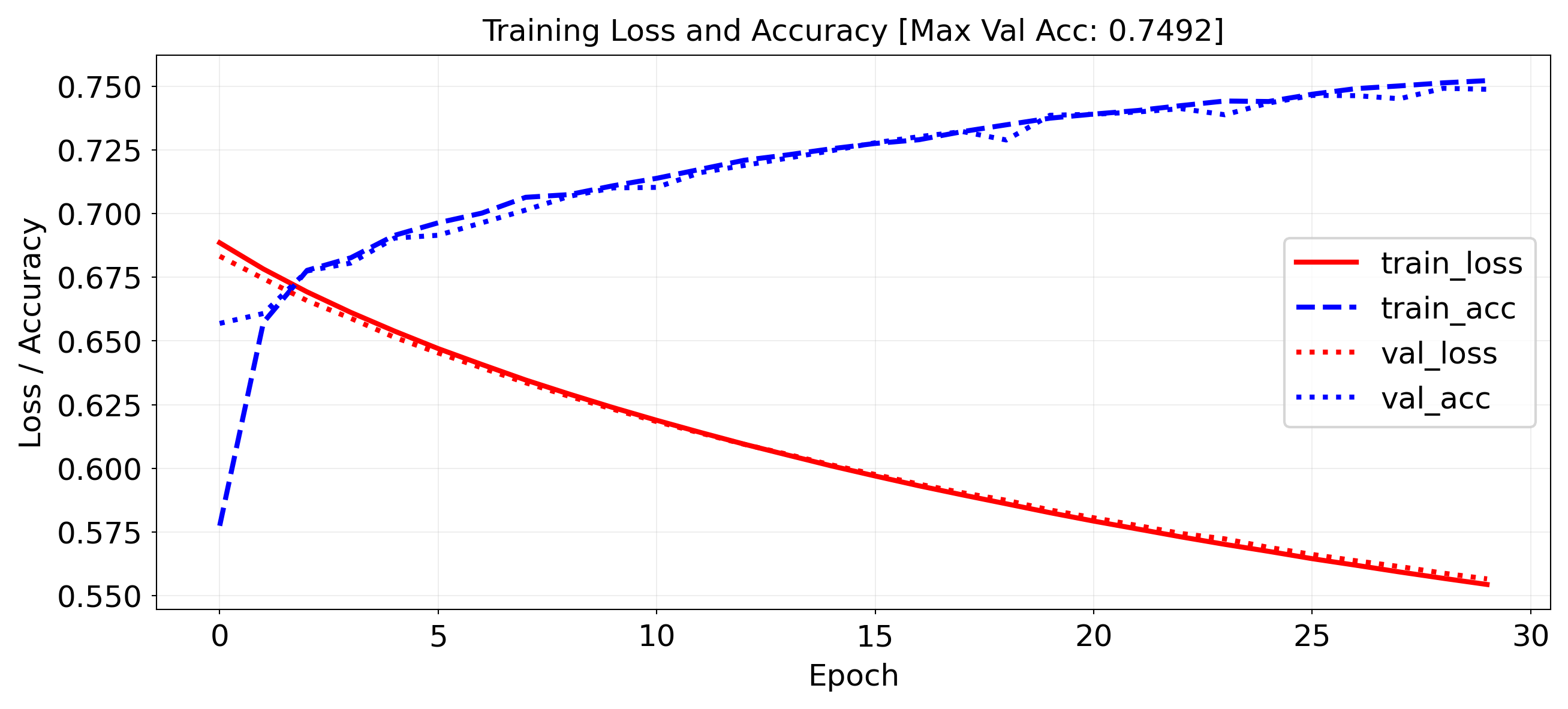
Same simple model, but with frozen GloVe embeddings: much worse!
Linear layer is too simple. We need something more complex -> transformers :)

embedding_tensor = torch.tensor(embedding_matrix, dtype=torch.float32)
self.model = nn.Sequential(
    nn.Embedding.from_pretrained(embedding_tensor, freeze=True),
    nn.AdaptiveAvgPool1d(1),
    nn.Linear(embedding_tensor.shape[1], 1))

# Load GloVe (assumes file is like 'glove.6B.300d.txt')
embedding_dim = 300
glove_path = "../data/glove.txt"

embeddings_index = {}
with open(glove_path, encoding='utf-8') as f:
    for line in f:
        values = line.strip().split()
        word = values[0]
        vector = np.asarray(values[1:], dtype='float32')
        embeddings_index[word] = vector
        
vocab_size = 10000
embedding_matrix = np.zeros((vocab_size, embedding_dim))
missing = 0

for word, i in word_index.items():
    if i < vocab_size:
        embedding_vector = embeddings_index.get(word)
        if embedding_vector is not None:
            embedding_matrix[i] = embedding_vector
        else:
            missing += 1

print(f"{missing} words not found in GloVe.")

class Permute(nn.Module):
    def __init__(self, *dims):
        super().__init__()
        self.dims = dims

    def forward(self, x):
        return x.permute(*self.dims)

class Squeeze(nn.Module):
    def __init__(self, dim=-1):
        super().__init__()
        self.dim = dim

    def forward(self, x):
        return x.squeeze(self.dim)

class FrozenGloVeModel(pl.LightningModule):
    def __init__(self, embedding_matrix, max_length=100):
        super().__init__()
        embedding_tensor = torch.tensor(embedding_matrix, dtype=torch.float32)

        self.model = nn.Sequential(
            nn.Embedding.from_pretrained(embedding_tensor, freeze=True),
            Permute(0, 2, 1),
            nn.AdaptiveAvgPool1d(1),
            Squeeze(dim=-1),
            nn.Linear(embedding_tensor.shape[1], 1),
            nn.Sigmoid()
        )

    def forward(self, x):
        return self.model(x).squeeze()

    def training_step(self, batch, batch_idx):
        x, y = batch
        y_hat = self(x)
        loss = F.binary_cross_entropy(y_hat, y)
        acc = ((y_hat > 0.5) == y.bool()).float().mean()
        self.log("train_loss", loss, on_step=False, on_epoch=True)
        self.log("train_acc", acc, on_step=False, on_epoch=True)
        return loss

    def validation_step(self, batch, batch_idx):
        x, y = batch
        y_hat = self(x)
        val_loss = F.binary_cross_entropy(y_hat, y)
        val_acc = ((y_hat > 0.5) == y.bool()).float().mean()
        self.log("val_loss", val_loss, on_epoch=True)
        self.log("val_acc", val_acc, on_epoch=True)

    def configure_optimizers(self):
        return torch.optim.Adam(self.parameters())
    
model = FrozenGloVeModel(embedding_matrix=embedding_matrix, max_length=100)

trainer = pl.Trainer(
    max_epochs=30,
    logger=False,
    enable_checkpointing=False,
    callbacks=[LivePlotCallback()]  # optional
)

trainer.fit(model, train_dataloaders=train_loader, val_dataloaders=val_loader)
        
        
        
        
        
        

../_images/3c08cdb7e86bcb1335bbf2d67a520121794913ce6be15f601d0e0e0e49f06981.png

`Trainer.fit` stopped: `max_epochs=30` reached.

Sequence-to-sequence (seq2seq) models#

Global average pooling or flattening destroys the word order
We need to model sequences explictly, e.g.:
- 1D convolutional models: run a 1D filter over the input data
  - Fast, but can only look at small part of the sentence
- Recurrent neural networks (RNNs)
  - Can look back at the entire previous sequence
  - Much slower to train, have limited memory in practice
- Attention-based networks (Transformers)
  - Best of both worlds: fast and very long memory

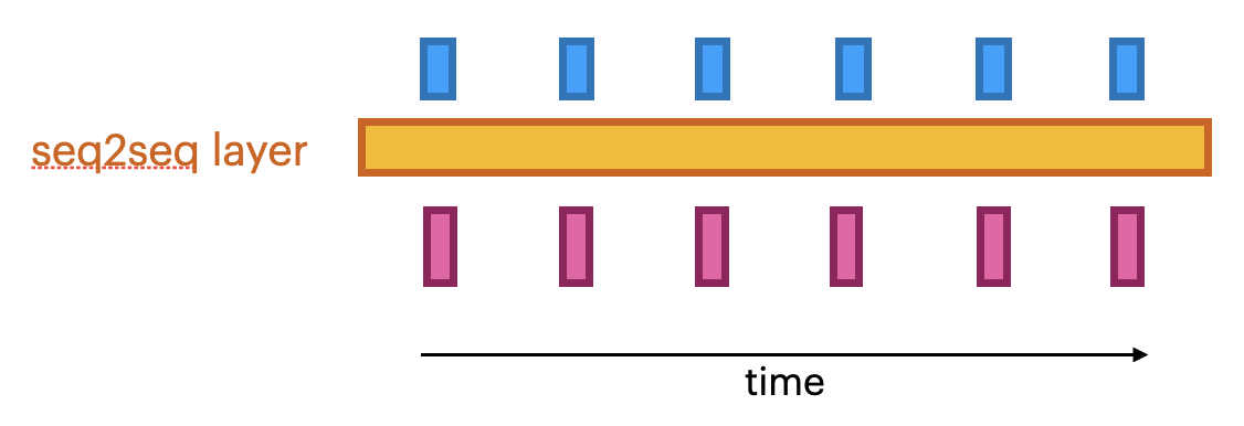
seq2seq models#

Produce a series of output given a series of inputs over time
Can handle sequences of different lengths
- Label-to-sequence, Sequence-to-label, seq2seq,…
- Autoregressive models (e.g. predict the next character, unsupervised)

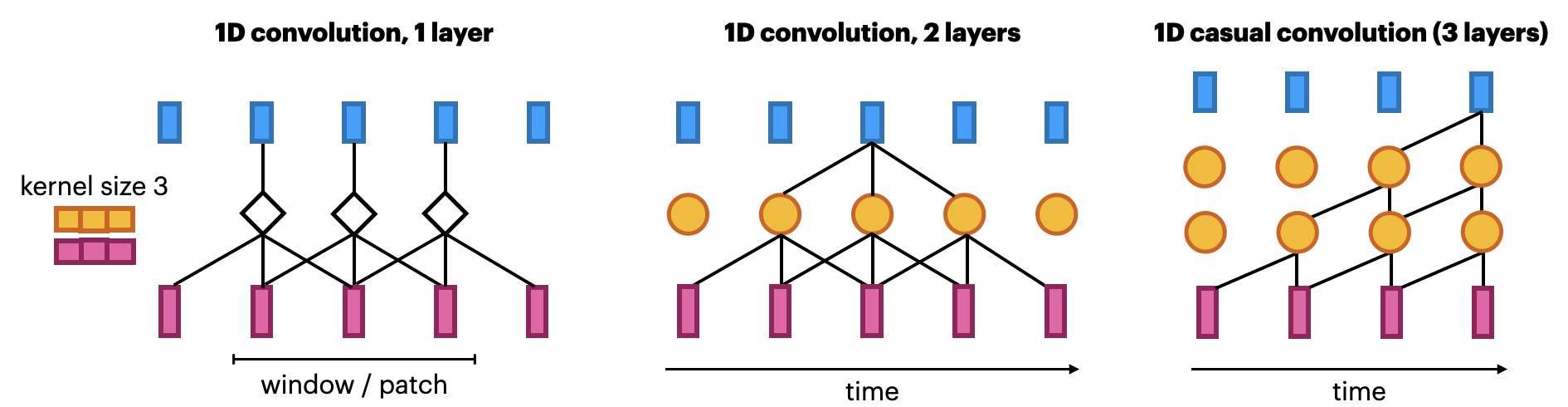
1D convolutional networks#

Similar to 2D convnets, but moves only in 1 direction (time)
- Extract local 1D patch, apply filter (kernel) to every patch
- Pattern learned can later be recognized elsewhere (translation invariance)
Limited memory: only sees a small part of the sequence (receptive field)
- You can use multiple layers, dilations,… but becomes expensive
Looks at ‘future’ parts of the series, but can be made to look only at the past
- Known as ‘causal’ models (not related to causality)

Same embedding, but add 2 Conv1D layers and MaxPooling1D.

model = nn.Sequential(
    nn.Embedding(num_embeddings=10000, embedding_dim=embedding_dim),
    nn.Conv1d(in_channels=embedding_dim, out_channels=32, kernel_size=7),
    nn.ReLU(),
    nn.MaxPool1d(kernel_size=5),
    nn.Conv1d(in_channels=32, out_channels=32, kernel_size=7),
    nn.ReLU(),
    nn.AdaptiveAvgPool1d(1),  # GAP
    nn.Flatten(),             # (batch, 32, 1) → (batch, 32)
    nn.Linear(32, 1)
)

model = nn.Sequential(
    nn.Embedding(num_embeddings=10000, embedding_dim=embedding_dim),  # embedding_layer
    nn.Conv1d(in_channels=embedding_dim, out_channels=32, kernel_size=7),
    nn.ReLU(),
    nn.MaxPool1d(kernel_size=5),
    nn.Conv1d(in_channels=32, out_channels=32, kernel_size=7),
    nn.ReLU(),
    nn.AdaptiveAvgPool1d(1),  # equivalent to GlobalAveragePooling1D
    nn.Flatten(),             # flatten (batch, 32, 1) → (batch, 32)
    nn.Linear(32, 1),
    nn.Sigmoid()
)

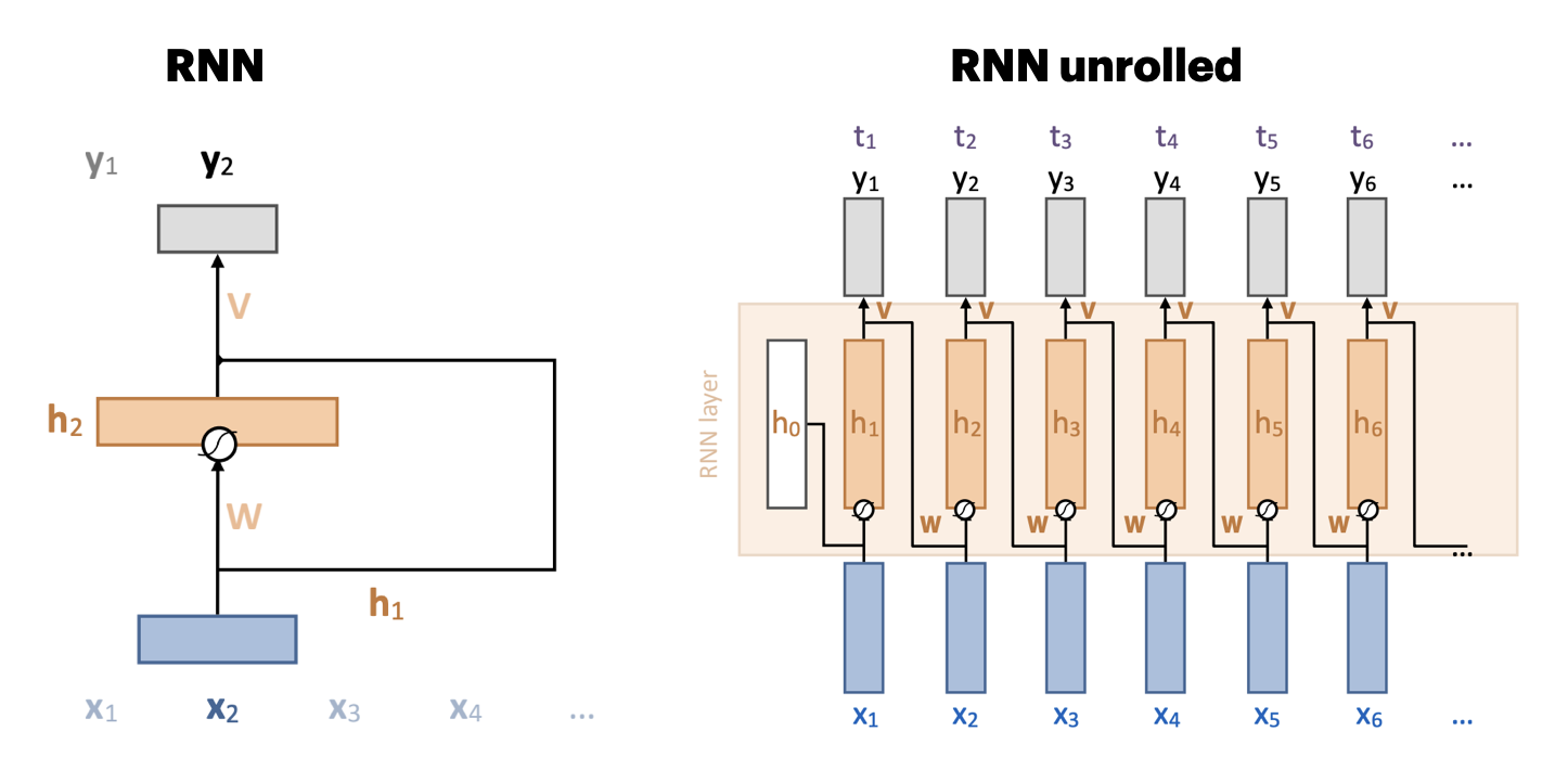
Recurrent neural networks (RNNs)#

Recurrent connection: concats output to next input ${\color{orange} h_t} = \sigma \left( {\color{orange} W } \left[ \begin{array}{c} {\color{blue}x}_t \\ {\color{orange} h}_{t-1} \end{array} \right] + b \right)$
Unbounded memory, but training requires backpropagation through time
- Requires storing previous network states (slow + lots of memory)
- Vanishing gradients strongly limit practical memory
Improved with gating: learn what to input, forget, output (LSTMs, GRUs,…)

Simple self-attention#

Maps a set of inputs to a set of outputs (without learned weigths)

Simple self-attention#

Compute dot product of input vector $x_i$ with every $x_j$ (including itself): ${\color{Orange} w_{ij}}$
Compute softmax over all these weights (positive, sum to 1)
Multiply by each input vector, and sum everything up
Can be easily vectorized: ${\color{green} Y}^T = {\color{orange} W}{\color{blue} X^T}$, ${\color{orange} W} = \textrm{softmax}( {\color{blue} X}^T {\color{blue}X} )$

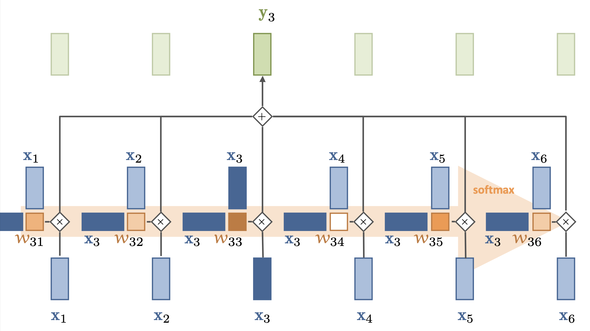
For each output, we mix information from all inputs according to how ‘similar’ they are
- The set of weights ${\color{Orange} w_{i}}$ for a given token is called the attention vector
- It says how much ‘attention’ each token gives to other tokens
Doesn’t learn (no parameters), the embedding of ${\color{blue} X}$ defines self-attention
- We’ll learn how to transform the embeddings later
- That way we can learn different relationships (not just similarity)
Has no problem looking very far back in the sequence
Operates on sets (permutation invariant): allows img-to-set, set-to-set,… tasks
- If the token order matters, we’ll have to encode it in the token embedding

Scaled dot products#

Self-attention is powerful because it’s mostly a linear operation
${\color{green} Y}^T = {\color{orange} W}{\color{blue} X^T}$ is linear, there are no vanishing gradients
- The softmax function only applies to ${\color{orange} W} = \textrm{softmax}( {\color{blue} X}^T {\color{blue}X} )$, not to ${\color{green} Y}^T$
- Needed to make the attention values sum up nicely to 1 without exploding
The dot products do get larger as the embedding dimension $k$ gets larger (by a factor $\sqrt{k}$)
- We therefore normalize the dot product by the input dimension $k$: ${\color{orange}w^{'}_{ij}} = \frac{{\color{blue} x_i}^T \color{blue} x_j}{\sqrt{k}}$
- This also makes training more stable: large softmas values lead to ‘sharp’ outputs, making some gradients very large and others very small

Simple self-attention layer#

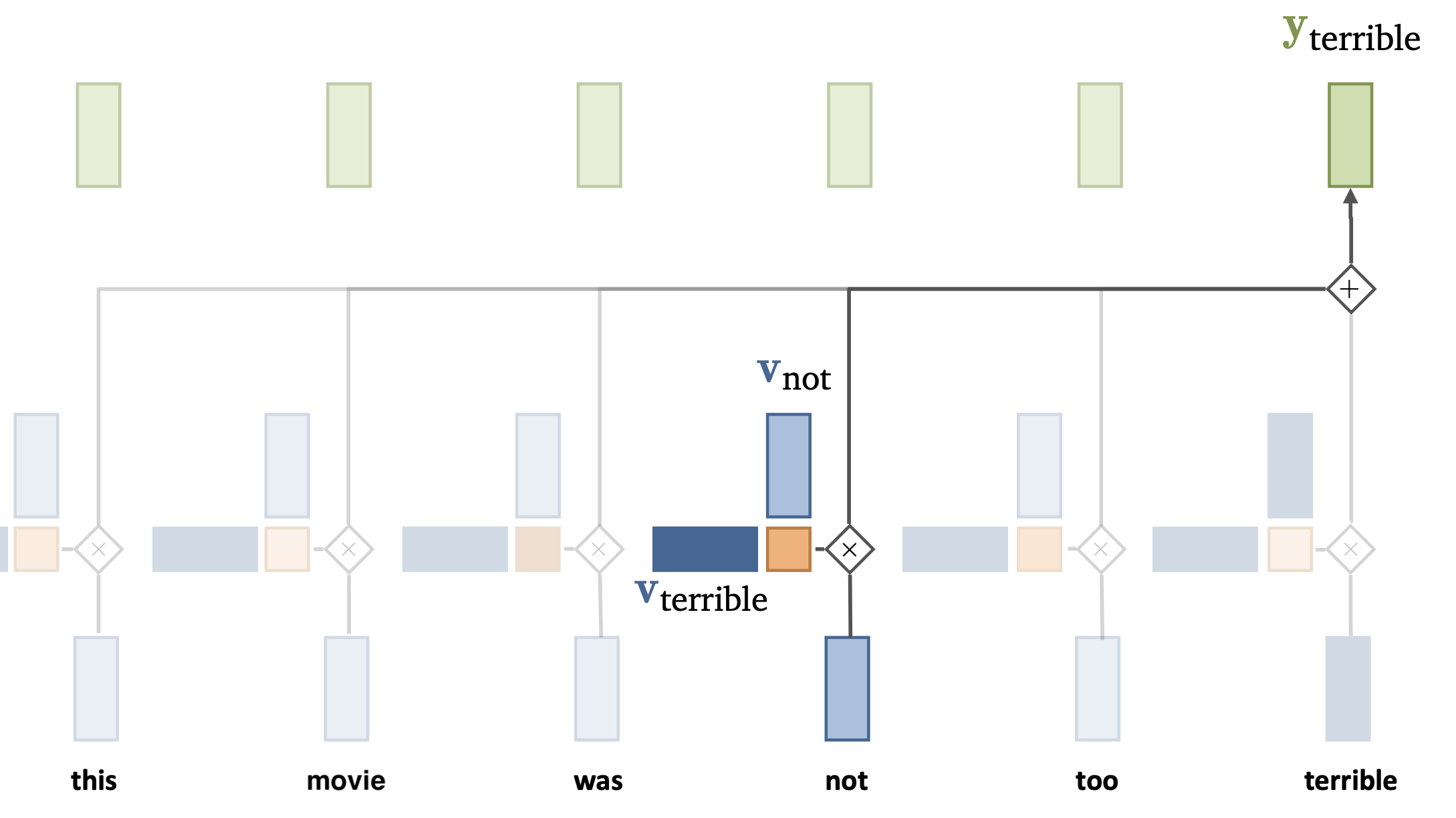
Let’s add a simple self-attention layer to our movie sentiment model
Without self-attention, every word would contribute independently (bag of words)
- The word terrible will likely result in a negative prediction
Now, we can freeze the embedding, take output ${\color{gray}Y}$, obtain a loss, and do backpropagation so that the self-attention layer can learn that ‘not’ should invert the meaning of ‘terrible’

Simple self-attention layer#

Through training, we want the self-attention to learn how certain tokens (e.g. ‘not’) can affect other tokens / words.
- E.g. we need to learn to change the representations of $v_{not}$ and $v_{terrible}$ so that they produce a ‘correct’ (low loss) output
For that, we do need to add some trainable parameters.

Standard self-attention#

We add 3 weight matrices (K, Q, V) and biases to change each vector:
- $k_i = K x_i + b_k$
- $q_i = Q x_i + b_q$
- $v_i = V x_i + b_v$
The same K, Q, V are used for all tokens depending on whether they are the input token (v), the token we are currently looking at (q), or the token we’re comparing with (k)

Sidenote on terminology#

View the set of tokens as a dictionary s = {a: v_a, b: v_b, c: v_c}
In a dictionary, the third output (for key c) would simple be s[c] = v_c
In a soft dictionary, it’s a weighted sum: $s[c] = w_a * v_a + w_b * v_b + w_c * v_c$
If $w_i$ are dot products: $s[c] = (k_a\cdot q_c) * v_a + (k_b\cdot q_c) * v_b + (k_b\cdot q_c) * v_c$
We blend the influence of every token based on their learned relations with other tokens

Intuition#

We blend the influence of every token based on their learned ‘relations’ with other tokens
Say that we need to learn how ‘negation’ works
- The ‘query’ vector could be trained (via Q) to say something like ‘are there any negation words?’
- A token (e.g. ‘not’), transformed by K, could then respond very positively if it is

Single-head self-attention#

There are different relations to model within a sentence.
The same input token, e.g. $v_{terrible}$ can relate completely differently to other kinds of tokens
- But we only have one set of K, V, and Q matrices
To better capture multiple relationships, we need multiple self-attention operations (expensive)

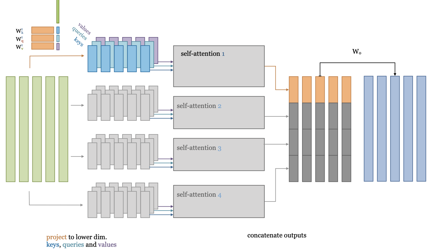
Multi-head self-attention#

What if we project the input embeddings to a lower-dimensional embedding $k$?
Then we could learn multiple self-attention operations in parallel
Effectively, we split the self-attention in multiple heads
- Each applies a separate low-dimensional self attention (with $K^{kxk},Q^{kxk},V^{kxk}$)
After running them (in parallel), we concatenate their outputs.

Transformer model#

Repeat self-attention multiple times in controlled fashion
Works for sequences, images, graphs,… (learn how sets of objects interact)
Models consist of multiple transformer blocks, usually:
- Layer normalization (every input is normalized independently)
- Self-attention layer (learn interactions)
- Residual connections (preserve gradients in deep networks)
- Feed-forward layer (learn mappings)

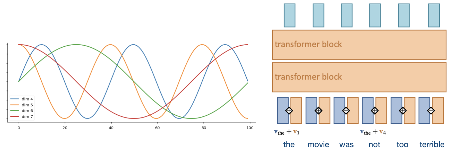
Positional encoding#

We need some way to tell the self-attention layer about position in the sequence
Represent position by vectors, using some easy-to-learn predictable pattern
- Add these encodings to vector embeddings
- Gives information on how far one input is from the others
Other techniques exist (e.g. relative positioning)

Autoregressive models#

Models that predict future values based on past values of the same stream
Output token is mapped to list of probabilities, sampled with softmax (with temperature)
Problem: self-attention can simply look ahead in the stream
- We need to make the transformer blocks causal

Masked self-attention#

Simple solution: simply mask out any attention weights from current to future tokens
Replace with -infinity, so that after softmax they will be 0

Famous transformers#

“Attention is all you need”: first paper to use attention without CNNs or RNNs
Encoder-Decoder architecture for translation: (k, q) to source attention layer
We’ll reproduce this (partly) in the Lab 6 tutorial :)

GPT 3#

Decoder-only, single stack of 96 transformer blocks (and 96 heads)
Sequence size 2048, input dimensionality 12,288, 175B parameters
Trained on entire common crawl dataset (1 epoch)
- Additional training on high-quality data (Wikipedia,…)
Excellent animation by 1b3b
GPT from scratch by A. Karpathy

GPT 4#

Likely a ‘mixtures of experts’ model
- Router (small MLP) selects which subnetworks (e.g. 2) to use given input
- Predictions get ensembled
Allows scaling up parameter count without proportionate (inference) cost
Also better data, more human-in-the-loop training (RLHF),…

Vision transformers#

Same principle: split up into patches, embed into tokens, add position encoding
For classification: add an extra (random) input token -> [CLS] output token

import torch
import torch.nn as nn
import torch.nn.functional as F
import torch.utils.data as data
import torch.optim as optim

## Torchvision
import torchvision
from torchvision.datasets import CIFAR10
from torchvision import transforms
import pytorch_lightning as pl
from pytorch_lightning.callbacks import LearningRateMonitor, ModelCheckpoint


device = "cpu"
if torch.backends.mps.is_available():
    device = "mps"
elif torch.cuda.is_available():
    device = "cuda"
print("Device:", device)

DATASET_PATH = "../data"
CHECKPOINT_PATH = "../data/checkpoints"

Device: mps

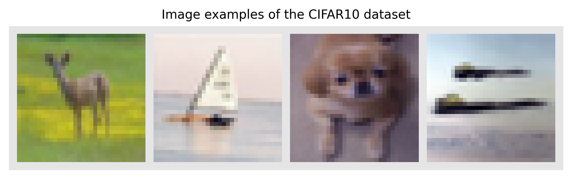
Demonstration#

We’ll experiment with the CIFAR-10 datasets

ViTs are quite expensive on large images.
This ViT takes about an hour to train (we’ll run it from a checkpoint)

pl.seed_everything(42)

Seed set to 42

from torchvision.transforms.autoaugment import AutoAugment, AutoAugmentPolicy
import multiprocessing
import copy

# Define normalization constants for CIFAR-10
CIFAR10_MEAN = [0.4914, 0.4822, 0.4465]
CIFAR10_STD = [0.2470, 0.2435, 0.2616]

# Define transforms. Using Auto-Augment
train_transform = transforms.Compose([
    AutoAugment(policy=AutoAugmentPolicy.CIFAR10),
    transforms.ToTensor(),
    transforms.Normalize(CIFAR10_MEAN, CIFAR10_STD),
])
# More aggressive, to reduce overfitting
train_transform = transforms.Compose([
    transforms.RandomCrop(32, padding=4),
    transforms.RandomHorizontalFlip(),
    transforms.ColorJitter(0.2, 0.2, 0.2, 0.1),
    transforms.ToTensor(),
    transforms.Normalize(CIFAR10_MEAN, CIFAR10_STD),
    transforms.RandomErasing(p=0.25)
])

test_transform = transforms.Compose([
    transforms.ToTensor(),
    transforms.Normalize(CIFAR10_MEAN, CIFAR10_STD),
])

# Load the full dataset once
full_dataset = CIFAR10(root=DATASET_PATH, train=True, download=True)
train_set, val_set = torch.utils.data.random_split(full_dataset, [45000, 5000])

# Apply different transforms to each split
train_set.dataset = copy.deepcopy(full_dataset)
train_set.dataset.transform = train_transform

val_set.dataset = copy.deepcopy(full_dataset)
val_set.dataset.transform = test_transform

# Load the test set
test_set = CIFAR10(root=DATASET_PATH, train=False, transform=test_transform, download=True)

# Optimized DataLoader settings
pin_memory = torch.cuda.is_available()
num_workers = multiprocessing.cpu_count()  # or set manually, e.g., 8

train_loader = data.DataLoader(
    train_set,
    batch_size=128,
    shuffle=True,
    drop_last=True,
    pin_memory=pin_memory,
    num_workers=num_workers,
    persistent_workers=True,
    prefetch_factor=4
)

val_loader = data.DataLoader(
    val_set,
    batch_size=128,
    shuffle=False,
    drop_last=False,
    pin_memory=pin_memory,
    num_workers=num_workers,
    persistent_workers=True,
    prefetch_factor=4
)

test_loader = data.DataLoader(
    test_set,
    batch_size=128,
    shuffle=False,
    drop_last=False,
    pin_memory=pin_memory,
    num_workers=num_workers,
    persistent_workers=True,
    prefetch_factor=4
)

# Visualize some examples
NUM_IMAGES = 4
CIFAR_images = torch.stack([val_set[idx][0] for idx in range(NUM_IMAGES)], dim=0)
img_grid = torchvision.utils.make_grid(CIFAR_images, nrow=4, normalize=True, pad_value=0.9)
img_grid = img_grid.permute(1, 2, 0)

plt.figure(figsize=(8,8))
plt.title("Image examples of the CIFAR10 dataset", fontsize=10)
plt.imshow(img_grid)
plt.axis('off')
plt.show()
plt.close()

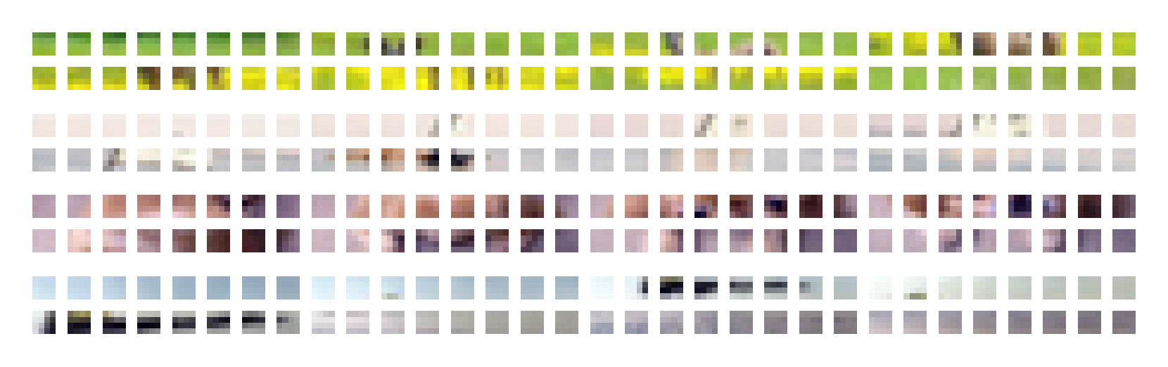
../_images/2dfa0f5fc605fb7b86f79d51ee0ccdfe23d626d2072b6e0df3a3f6523d1d48c6.png

Patchify#

Split $N\times N$ image into $(N/M)^2$ patches of size $M\times M$.

    B, C, H, W = x.shape  # Batch size, Channels, Height, Width
    x = x.reshape(B, C, H//patch_size, patch_size, W//patch_size, patch_size)

def img_to_patch(x, patch_size, flatten_channels=True):
    """
    Inputs:
        x - torch.Tensor representing the image of shape [B, C, H, W]
        patch_size - Number of pixels per dimension of the patches (integer)
        flatten_channels - If True, the patches will be returned in a flattened format
                           as a feature vector instead of a image grid.
    """
    B, C, H, W = x.shape
    x = x.reshape(B, C, H//patch_size, patch_size, W//patch_size, patch_size)
    x = x.permute(0, 2, 4, 1, 3, 5) # [B, H', W', C, p_H, p_W]
    x = x.flatten(1,2)              # [B, H'*W', C, p_H, p_W]
    if flatten_channels:
        x = x.flatten(2,4)          # [B, H'*W', C*p_H*p_W]
    return x

img_patches = img_to_patch(CIFAR_images, patch_size=4, flatten_channels=False)

fig, ax = plt.subplots(CIFAR_images.shape[0], 1, figsize=(14, 2))
for i in range(CIFAR_images.shape[0]):
    img_grid = torchvision.utils.make_grid(img_patches[i], nrow=32, normalize=True, pad_value=1)
    img_grid = img_grid.permute(1, 2, 0)
    ax[i].imshow(img_grid)
    ax[i].axis('off')

plt.subplots_adjust(hspace=0)  # Reduce vertical spacing between rows
plt.show()
plt.close()

../_images/23830748dd5bf02ee22453ce729e6beb6849bc112addc808eb80460c397e23ec.png

Self-attention#

First, we need to implement a (scaled) dot-product

Self-attention#

First, we need to implement a (scaled) dot-product

def scaled_dot_product(q, k, v):
    attn_logits = torch.matmul(q, k.transpose(-2, -1)) # dot prod
    attn_logits = attn_logits / math.sqrt(q.size()[-1])# scaling
    attention = F.softmax(attn_logits, dim=-1)         # softmax
    values = torch.matmul(attention, v)                # dot prod
    return values, attention

def scaled_dot_product(q, k, v, mask=None):
    d_k = q.size()[-1]
    attn_logits = torch.matmul(q, k.transpose(-2, -1))
    attn_logits = attn_logits / math.sqrt(d_k)
    if mask is not None:
        attn_logits = attn_logits.masked_fill(mask == 0, -9e15)
    attention = F.softmax(attn_logits, dim=-1)
    values = torch.matmul(attention, v)
    return values, attention

Multi-head attention (simplified)#

Project input to lower-dimensional embeddings
Stack them so we can feed them through self-attention at once
Unstack and project back to original dimensions

    qkv = nn.Linear(input_dim, 3*embed_dim)(x) # project to embed_dim
    qkv = qkv.reshape(batch_size, seq_length, num_heads, 3*head_dim)
    q, k, v = qkv.chunk(3, dim=-1) 

    values, attention = scaled_dot_product(q, k, v, mask=mask) # self-att
    values = values.reshape(batch_size, seq_length, embed_dim)
    out = nn.Linear(embed_dim, input_dim) # project back

def expand_mask(mask):
    assert mask.ndim >= 2, "Mask must be at least 2-dimensional with seq_length x seq_length"
    if mask.ndim == 3:
        mask = mask.unsqueeze(1)
    while mask.ndim < 4:
        mask = mask.unsqueeze(0)
    return mask

class MultiheadAttention(nn.Module):
    
    def __init__(self, input_dim, embed_dim, num_heads):
        super().__init__()
        assert embed_dim % num_heads == 0, "Embedding dimension must be 0 modulo number of heads."
        
        self.embed_dim = embed_dim
        self.num_heads = num_heads
        self.head_dim = embed_dim // num_heads
        
        # Stack all weight matrices 1...h together for efficiency
        # Note that in many implementations you see "bias=False" which is optional
        self.qkv_proj = nn.Linear(input_dim, 3*embed_dim)
        self.o_proj = nn.Linear(embed_dim, input_dim)
        
        self._reset_parameters()

    def _reset_parameters(self):
        # Original Transformer initialization, see PyTorch documentation
        nn.init.xavier_uniform_(self.qkv_proj.weight)
        self.qkv_proj.bias.data.fill_(0)
        nn.init.xavier_uniform_(self.o_proj.weight)
        self.o_proj.bias.data.fill_(0)

    def forward(self, x, mask=None, return_attention=False):
        batch_size, seq_length, _ = x.size()
        if mask is not None:
            mask = expand_mask(mask)
        qkv = self.qkv_proj(x)
        
        # Separate Q, K, V from linear output
        qkv = qkv.reshape(batch_size, seq_length, self.num_heads, 3*self.head_dim)
        qkv = qkv.permute(0, 2, 1, 3) # [Batch, Head, SeqLen, Dims]
        q, k, v = qkv.chunk(3, dim=-1)
        
        # Determine value outputs
        values, attention = scaled_dot_product(q, k, v, mask=mask)
        values = values.permute(0, 2, 1, 3) # [Batch, SeqLen, Head, Dims]
        values = values.reshape(batch_size, seq_length, self.embed_dim)
        o = self.o_proj(values)
        
        if return_attention:
            return o, attention
        else:
            return o

Attention block#

The attention block is quite straightforward

Attention block#

def __init__(self, embed_dim, hidden_dim, num_heads, dropout=0.0):
    self.layer_norm_1 = nn.LayerNorm(embed_dim)
    self.attn = nn.MultiheadAttention(embed_dim, num_heads)
    self.layer_norm_2 = nn.LayerNorm(embed_dim)
    self.linear = nn.Sequential( # Feed-forward layer
        nn.Linear(embed_dim, hidden_dim),
        nn.GELU(), nn.Dropout(dropout),
        nn.Linear(hidden_dim, embed_dim),
        nn.Dropout(dropout)
    )

def forward(self, x):
    inp_x = self.layer_norm_1(x)
    x = x + self.attn(inp_x, inp_x, inp_x)[0] # self-att + res
    x = x + self.linear(self.layer_norm_2(x)) # feed-fw + res
    return x

class AttentionBlock(nn.Module):
    
    def __init__(self, embed_dim, hidden_dim, num_heads, dropout=0.0):
        """
        Inputs:
            embed_dim - Dimensionality of input and attention feature vectors
            hidden_dim - Dimensionality of hidden layer in feed-forward network 
                         (usually 2-4x larger than embed_dim)
            num_heads - Number of heads to use in the Multi-Head Attention block
            dropout - Amount of dropout to apply in the feed-forward network
        """
        super().__init__()
        
        self.layer_norm_1 = nn.LayerNorm(embed_dim)
        self.attn = nn.MultiheadAttention(embed_dim, num_heads, 
                                          dropout=dropout)
        self.layer_norm_2 = nn.LayerNorm(embed_dim)
        self.linear = nn.Sequential(
            nn.Linear(embed_dim, hidden_dim),
            nn.GELU(),
            nn.Dropout(dropout),
            nn.Linear(hidden_dim, embed_dim),
            nn.Dropout(dropout)
        )
        
        
    def forward(self, x):
        inp_x = self.layer_norm_1(x)
        x = x + self.attn(inp_x, inp_x, inp_x)[0]
        x = x + self.linear(self.layer_norm_2(x))
        return x

Vision transformer#

Final steps:

Linear projection (embedding) to map patches to vector
Add classification token to input
2D positional encoding
Small MLP head to map CLS token to prediction

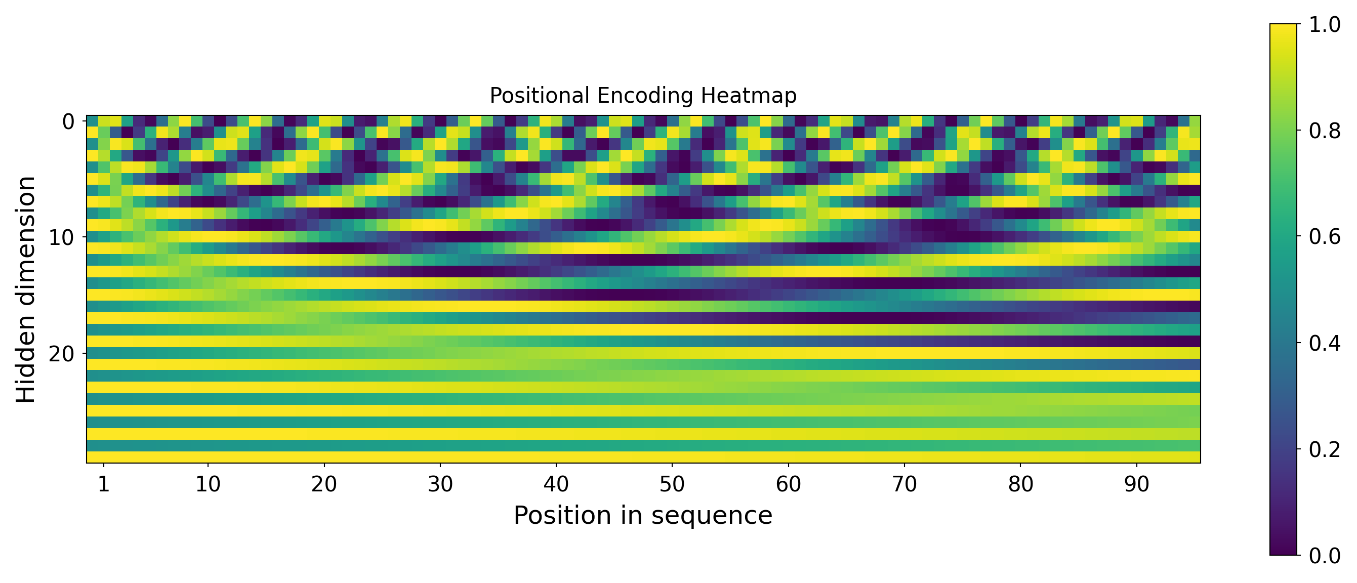
Positional encoding#

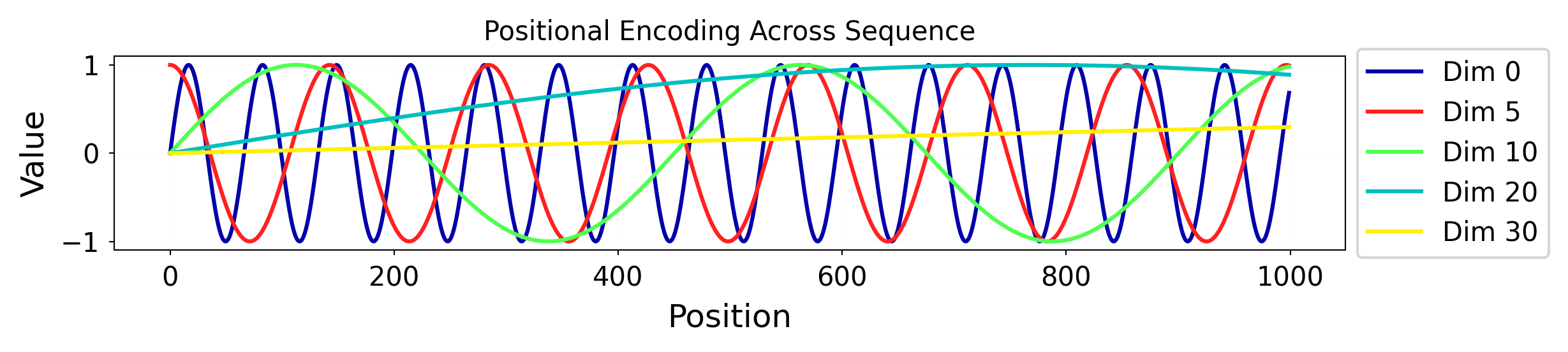
We implement this pattern and run in across a 2D grid: $$ PE_{(pos,i)} = \begin{cases} \sin\left(\frac{pos}{10000^{i/d_{\text{model}}}}\right) & \text{if}\hspace{3mm} i \text{ mod } 2=0\\ \cos\left(\frac{pos}{10000^{(i-1)/d_{\text{model}}}}\right) & \text{otherwise}\\ \end{cases} $$

from sklearn.preprocessing import MinMaxScaler
import math

plt.rcParams.update({
    'font.size': 12,
    'axes.labelsize': 12,
    'axes.titlesize': 10,
    'xtick.labelsize': 10,
    'ytick.labelsize': 10,
    'legend.fontsize': 10,
    'lines.linewidth': 1.5
})

class PositionalEncoding(nn.Module):
    def __init__(self, d_model, max_len=5000):
        super().__init__()
        pe = torch.zeros(max_len, d_model)
        position = torch.arange(0, max_len, dtype=torch.float).unsqueeze(1)
        div_term = torch.exp(torch.arange(0, d_model, 2).float() * (-math.log(10000.0) / d_model))
        pe[:, 0::2] = torch.sin(position * div_term)
        pe[:, 1::2] = torch.cos(position * div_term)
        pe = pe.unsqueeze(0)
        self.register_buffer('pe', pe, persistent=False)

    def forward(self, x):
        return x + self.pe[:, :x.size(1)]

# Create positional encoding
d_model = 48
max_len = 96
encod_block = PositionalEncoding(d_model=d_model, max_len=max_len)
pe = encod_block.pe.squeeze().T.cpu().numpy()  # Shape: [d_model, max_len]

# Global normalization
pe_subset = pe[:30]
pe_norm = (pe_subset - pe_subset.min()) / (pe_subset.max() - pe_subset.min())

# Plot heatmap with global normalization
fig, ax = plt.subplots(figsize=(10, 4))
img = ax.imshow(pe_norm, cmap="viridis")
fig.colorbar(img, ax=ax)
ax.set_xlabel("Position in sequence")
ax.set_ylabel("Hidden dimension")
ax.set_title("Positional Encoding Heatmap")
ax.set_xticks([1] + [i*10 for i in range(1, 1 + pe.shape[1]//10)])
ax.set_yticks(np.arange(0, 30, 10))
ax.set_yticklabels([str(i) for i in range(0, 30, 10)])
plt.tight_layout()
plt.show()

# Smooth 1D plot for selected dimensions
high_res_positions = torch.linspace(0, max_len - 1, steps=1000).unsqueeze(1)
div_term = torch.exp(torch.arange(0, d_model, 2).float() * (-math.log(10000.0) / d_model))
pe_highres = torch.zeros((1000, d_model))
pe_highres[:, 0::2] = torch.sin(high_res_positions * div_term)
pe_highres[:, 1::2] = torch.cos(high_res_positions * div_term)
pe_highres_np = pe_highres.T.cpu().numpy()

plt.figure(figsize=(10, 2))
for i in [0, 5, 10, 20, 30]:
    plt.plot(pe_highres_np[i], linestyle='-', label=f"Dim {i}")
plt.title("Positional Encoding Across Sequence")
plt.xlabel("Position")
plt.ylabel("Value")
plt.legend(loc='center left', bbox_to_anchor=(1.01, 0.5), borderaxespad=0.)
plt.grid(True, linestyle='--', alpha=0.3)
plt.tight_layout(rect=[0, 0, 0.85, 1])
plt.show()

../_images/7014978cdab4c25d47df3be2c8bee2c6842439e2c1d063e9a78dd416b0b0d16c.png

../_images/5f054010c084fc46f6e458fdb1188edcf75f369c4f95ff6bbf093efbdc5ef9d3.png

class VisionTransformer(nn.Module):
    
    def __init__(self, embed_dim, hidden_dim, num_channels, num_heads, num_layers, num_classes, patch_size, num_patches, dropout=0.0):
        """
        Inputs:
            embed_dim - Dimensionality of the input feature vectors to the Transformer
            hidden_dim - Dimensionality of the hidden layer in the feed-forward networks
                         within the Transformer
            num_channels - Number of channels of the input (3 for RGB)
            num_heads - Number of heads to use in the Multi-Head Attention block
            num_layers - Number of layers to use in the Transformer
            num_classes - Number of classes to predict
            patch_size - Number of pixels that the patches have per dimension
            num_patches - Maximum number of patches an image can have
            dropout - Amount of dropout to apply in the feed-forward network and 
                      on the input encoding
        """
        super().__init__()
        
        self.patch_size = patch_size
        
        # Layers/Networks
        self.input_layer = nn.Linear(num_channels*(patch_size**2), embed_dim)
        self.transformer = nn.Sequential(*[AttentionBlock(embed_dim, hidden_dim, num_heads, dropout=dropout) for _ in range(num_layers)])
        self.mlp_head = nn.Sequential(
            nn.LayerNorm(embed_dim),
            nn.Linear(embed_dim, num_classes)
        )
        self.dropout = nn.Dropout(dropout)
        
        # Parameters/Embeddings
        self.cls_token = nn.Parameter(torch.randn(1,1,embed_dim))
        self.pos_embedding = nn.Parameter(torch.randn(1,1+num_patches,embed_dim))
    
    
    def forward(self, x):
        # Preprocess input
        x = img_to_patch(x, self.patch_size)
        B, T, _ = x.shape
        x = self.input_layer(x)
        
        # Add CLS token and positional encoding
        cls_token = self.cls_token.repeat(B, 1, 1)
        x = torch.cat([cls_token, x], dim=1)
        x = x + self.pos_embedding[:,:T+1]
        
        # Apply Transforrmer
        x = self.dropout(x)
        x = x.transpose(0, 1)
        x = self.transformer(x)
        
        # Perform classification prediction
        cls = x[0]
        out = self.mlp_head(cls)
        return out

class ViT(pl.LightningModule):
    
    def __init__(self, model_kwargs, lr):
        super().__init__()
        self.save_hyperparameters()
        self.model = VisionTransformer(**model_kwargs)
        self.example_input_array = next(iter(train_loader))[0]
        
    def forward(self, x):
        return self.model(x)
    
    def configure_optimizers(self):
        optimizer = optim.AdamW(self.parameters(), lr=self.hparams.lr)
        lr_scheduler = optim.lr_scheduler.MultiStepLR(optimizer, milestones=[100,150], gamma=0.1)
        return [optimizer], [lr_scheduler]   
    
    def _calculate_loss(self, batch, mode="train"):
        imgs, labels = batch
        preds = self.model(imgs)
        loss = F.cross_entropy(preds, labels)
        acc = (preds.argmax(dim=-1) == labels).float().mean()
        
        self.log(f'{mode}_loss', loss)
        self.log(f'{mode}_acc', acc)
        return loss

    def training_step(self, batch, batch_idx):
        loss = self._calculate_loss(batch, mode="train")
        return loss

    def validation_step(self, batch, batch_idx):
        self._calculate_loss(batch, mode="val")

    def test_step(self, batch, batch_idx):
        self._calculate_loss(batch, mode="test")
        
from torchvision.models import resnet18

class ResNet18Classifier(pl.LightningModule):
    def __init__(self, num_classes, lr):
        super().__init__()
        self.save_hyperparameters()
        base_model = resnet18(weights=None)
        in_features = base_model.fc.in_features
        base_model.fc = nn.Sequential(
            nn.Dropout(p=0.3),
            nn.Linear(in_features, num_classes)
        )
        self.model = base_model
        self.example_input_array = next(iter(train_loader))[0]
    
    def forward(self, x):
        return self.model(x)
    
    def configure_optimizers(self):
        optimizer = optim.AdamW(self.parameters(), lr=self.hparams.lr, weight_decay=1e-4)
        lr_scheduler = optim.lr_scheduler.MultiStepLR(optimizer, milestones=[100, 150], gamma=0.1)
        return [optimizer], [lr_scheduler]
    
    def _calculate_loss(self, batch, mode="train"):
        imgs, labels = batch
        preds = self(imgs)
        loss = F.cross_entropy(preds, labels, label_smoothing=0.1)
        acc = (preds.argmax(dim=-1) == labels).float().mean()

        self.log(f'{mode}_loss', loss)
        self.log(f'{mode}_acc', acc)
        return loss
    
    def training_step(self, batch, batch_idx):
        return self._calculate_loss(batch, mode="train")

    def validation_step(self, batch, batch_idx):
        self._calculate_loss(batch, mode="val")

    def test_step(self, batch, batch_idx):
        self._calculate_loss(batch, mode="test")

from matplotlib.cm import get_cmap
from IPython.display import display, update_display

class LiveCompareCallback(pl.Callback):
    def __init__(self, history, model_name):
        self.history = history
        self.model_name = model_name
        self.max_val_acc = 0
        self.display_id = None  # For live plot replacement
        self.display_handle = None

        if "_colors" not in self.history:
            self.history["_colors"] = {}
        if model_name not in self.history["_colors"]:
            cmap = plt.get_cmap("tab10")
            color_idx = len(self.history["_colors"])
            self.history["_colors"][model_name] = cmap(color_idx % 10)

        if model_name not in self.history:
            self.history[model_name] = {
                "train_loss": [],
                "train_acc": [],
                "val_loss": [],
                "val_acc": []
            }

    def on_train_epoch_end(self, trainer, pl_module):
        metrics = trainer.callback_metrics
        train_loss = metrics.get("train_loss")
        train_acc = metrics.get("train_acc")
        val_loss = metrics.get("val_loss")
        val_acc = metrics.get("val_acc")

        if all(v is not None for v in [train_loss, train_acc, val_loss, val_acc]):
            self.history[self.model_name]["train_loss"].append(train_loss.item())
            self.history[self.model_name]["train_acc"].append(train_acc.item())
            self.history[self.model_name]["val_loss"].append(val_loss.item())
            self.history[self.model_name]["val_acc"].append(val_acc.item())
            self.max_val_acc = max(self.max_val_acc, val_acc.item())
            self.plot_all_models()

    def plot_all_models(self):
        fig, axes = plt.subplots(1, 2, figsize=(12, 5))

        for model_name, logs in self.history.items():
            if model_name == "_colors":
                continue
            color = self.history["_colors"][model_name]
            epochs = range(len(logs["train_loss"]))

            axes[0].plot(epochs, logs["train_loss"], label=f'{model_name} Train', linestyle='-', color=color)
            axes[0].plot(epochs, logs["val_loss"], label=f'{model_name} Val', linestyle=':', color=color)

            axes[1].plot(epochs, logs["train_acc"], label=f'{model_name} Train', linestyle='-', color=color)
            axes[1].plot(epochs, logs["val_acc"], label=f'{model_name} Val', linestyle=':', color=color)

        axes[0].set_title("Loss", fontsize=10)
        axes[1].set_title("Accuracy", fontsize=10)
        for ax in axes:
            ax.set_xlabel("Epoch", fontsize=10)
            ax.grid(True)
            ax.legend()
        axes[0].set_ylabel("Loss", fontsize=10)
        axes[1].set_ylabel("Accuracy", fontsize=10)
        plt.suptitle("Model Comparison", fontsize=14)
        plt.tight_layout()

        # Display once, then update in-place
        if self.display_handle is None:
            self.display_handle = display(fig, display_id=True)
        else:
            self.display_handle.update(fig)

        plt.close(fig)

def train_model(model_class, model_name, model_kwargs, lr, history):
    model_ckpt_path = os.path.join(CHECKPOINT_PATH, model_name)
    pretrained_filename = os.path.join(model_ckpt_path, f"{model_name}.ckpt")

    callback = LiveCompareCallback(history=history, model_name=model_name)

    trainer = pl.Trainer(
        default_root_dir=model_ckpt_path,
        accelerator="auto",
        devices=1,
        max_epochs=50,
        callbacks=[
            ModelCheckpoint(save_weights_only=True, mode="max", monitor="val_acc"),
            LearningRateMonitor("epoch"),
            callback
        ],
        logger=pl.loggers.TensorBoardLogger(save_dir=model_ckpt_path, name=model_name)
    )

    if os.path.isfile(pretrained_filename):
        print(f"Found pretrained model at {pretrained_filename}, loading...")
        model = model_class.load_from_checkpoint(pretrained_filename)
    else:
        pl.seed_everything(42)
        model = model_class(**model_kwargs, lr=lr)
        trainer.fit(model, train_loader, val_loader)
        model = model_class.load_from_checkpoint(trainer.checkpoint_callback.best_model_path)

    val_result = trainer.test(model, val_loader, verbose=False)
    test_result = trainer.test(model, test_loader, verbose=False)

    return model, {
        "val": val_result[0]["test_acc"],
        "test": test_result[0]["test_acc"]
    }

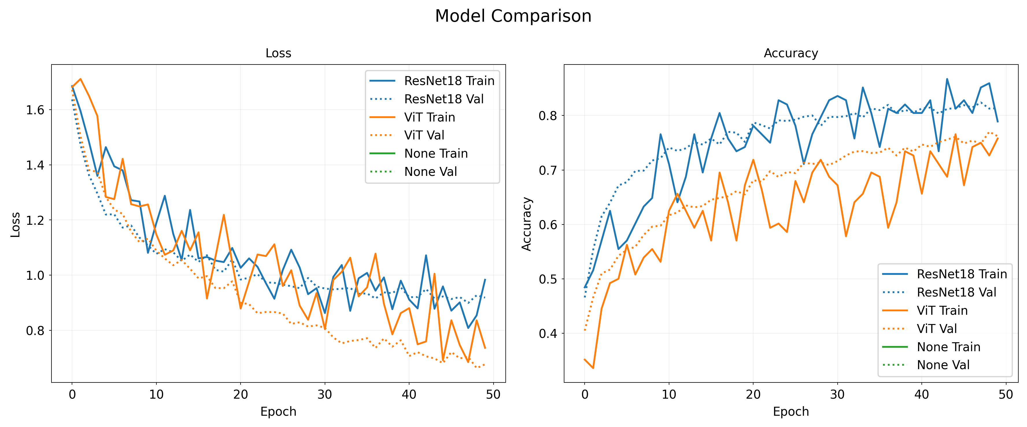
Results#

ResNet outperforms ViT!
Inductive biases of CNNs win out if you have limited data/compute
Transformers have very little inductive bias
- More flexible, but also more data hungry

with open("../data/vit_histories.pkl", "rb") as f:
    histories = pickle.load(f)

if "vit" in histories:
    lccb = LiveCompareCallback(histories["vit"], None)
    lccb.plot_all_models()
else: 
    vit_kwargs={'embed_dim': 256,
                'hidden_dim': 512,
                'num_heads': 8,
                'num_layers': 6,
                'patch_size': 4,
                'num_channels': 3,
                'num_patches': 64,
                'num_classes': 10,
                'dropout': 0.2}

    history = {}

    resnet_model, resnet_results = train_model(
        model_class=ResNet18Classifier,
        model_name="ResNet18",
        model_kwargs={"num_classes": 10},
        lr=3e-4,
        history=history
    )

    vit_model, vit_results = train_model(
        model_class=ViT,
        model_name="ViT",
        model_kwargs={"model_kwargs": vit_kwargs},
        lr=3e-4,
        history=history
    )

../_images/573a0be76a66288dd6dc219049ddf41723aa427547379fd2f835921b8d8b4e2f.png

# Store history
import pickle 

if "vit" not in histories:
    histories = {"vit":history}
    with open("../data/vit_histories.pkl", "wb") as f:
        pickle.dump(histories, f)

Summary#

Tokenization
- Find a good way to split data into tokens
Word/Image embeddings (for initial embeddings)
- For text: Word2Vec, FastText, GloVe
- For images: MLP, CNN,…
Sequence-to-sequence models
- 1D convolutional nets (fast, limited memory)
- RNNs (slow, also quite limited memory)
Transformers
- Self-attention (allows very large memory)
- Positional encoding
- Autoregressive models
Vision transformers
- Useful if you have lots of data (and compute)

Acknowledgement

Several figures came from the excellent VU Deep Learning course.

Lecture 8. Transformers

Contents

Lecture 8. Transformers#

Overview#

Bag of word representation#

Text preprocessing pipelines#

Scaling#

Neural networks on bag of words#

Evaluation#

Predictions#

Word Embeddings#

Learning embeddings from scratch#

Pre-trained embeddings#

Word2Vec#

Word2Vec properties#

Doc2Vec#

FastText#

Global Vector model (GloVe)#

Sequence-to-sequence (seq2seq) models#

seq2seq models#

1D convolutional networks#

Recurrent neural networks (RNNs)#

Simple self-attention#

Simple self-attention#

Scaled dot products#

Simple self-attention layer#

Simple self-attention layer#

Standard self-attention#

Sidenote on terminology#

Intuition#

Single-head self-attention#

Multi-head self-attention#

Transformer model#

Positional encoding#

Autoregressive models#

Masked self-attention#

Famous transformers#

GPT 3#

GPT 4#

Vision transformers#

Demonstration#

Patchify#

Self-attention#

Self-attention#

Multi-head attention (simplified)#

Attention block#

Attention block#

Vision transformer#

Positional encoding#

Results#

Summary#