
Lecture 2. Linear models#
Basics of modeling, optimization, and regularization
Joaquin Vanschoren
Show code cell source
# Auto-setup when running on Google Colab
import os
if 'google.colab' in str(get_ipython()) and not os.path.exists('/content/master'):
    !git clone -q https://github.com/ML-course/master.git /content/master
    !pip --quiet install -r /content/master/requirements_colab.txt
    %cd master/notebooks

# Global imports and settings
%matplotlib inline
from preamble import *
interactive = False # Set to True for interactive plots
if interactive:
    fig_scale = 0.5
    plt.rcParams.update(print_config)
else: # For printing
    fig_scale = 0.3
    plt.rcParams.update(print_config)
Notation and Definitions#
A scalar is a simple numeric value, denoted by an italic letter: \(x=3.24\)
A vector is a 1D ordered array of n scalars, denoted by a bold letter: \(\mathbf{x}=[3.24, 1.2]\)
\(x_i\) denotes the \(i\)th element of a vector, thus \(x_0 = 3.24\).
Note: some other courses use \(x^{(i)}\) notation
A set is an unordered collection of unique elements, denote by caligraphic capital: \(\mathcal{S}=\{3.24, 1.2\}\)
A matrix is a 2D array of scalars, denoted by bold capital: \(\mathbf{X}=\begin{bmatrix} 3.24 & 1.2 \\ 2.24 & 0.2 \end{bmatrix}\)
\(\textbf{X}_{i}\) denotes the \(i\)th row of the matrix
\(\textbf{X}_{:,j}\) denotes the \(j\)th column
\(\textbf{X}_{i,j}\) denotes the element in the \(i\)th row, \(j\)th column, thus \(\mathbf{X}_{1,0} = 2.24\)
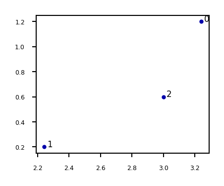
\(\mathbf{X}^{n \times p}\), an \(n \times p\) matrix, can represent \(n\) data points in a \(p\)-dimensional space
Every row is a vector that can represent a point in an p-dimensional space, given a basis.
The standard basis for a Euclidean space is the set of unit vectors
E.g. if \(\mathbf{X}=\begin{bmatrix} 3.24 & 1.2 \\ 2.24 & 0.2 \\ 3.0 & 0.6 \end{bmatrix}\)
Show code cell source
X = np.array([[3.24 , 1.2 ],[2.24, 0.2],[3.0 , 0.6 ]])
fig = plt.figure(figsize=(5*fig_scale,4*fig_scale))
plt.scatter(X[:,0],X[:,1]);
for i in range(3):
    plt.annotate(i, (X[i,0]+0.02, X[i,1]))
A tensor is an k-dimensional array of data, denoted by an italic capital: \(T\)
k is also called the order, degree, or rank
\(T_{i,j,k,...}\) denotes the element or sub-tensor in the corresponding position
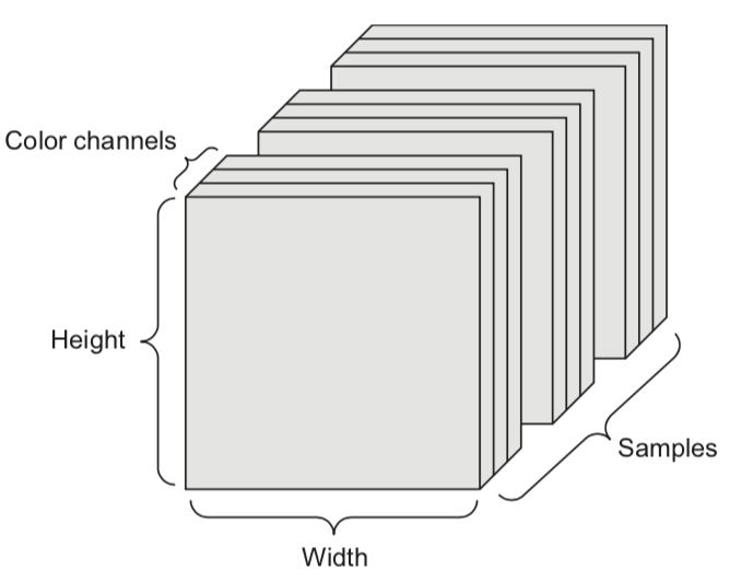
A set of color images can be represented by:
a 4D tensor (sample x height x width x color channel)
a 2D tensor (sample x flattened vector of pixel values)
Basic operations#
Sums and products are denoted by capital Sigma and capital Pi:
Operations on vectors are element-wise: e.g. \(\mathbf{x}+\mathbf{z} = [x_0+z_0,x_1+z_1, ... , x_p+z_p]\)
Dot product \(\mathbf{w}\mathbf{x} = \mathbf{w} \cdot \mathbf{x} = \mathbf{w}^{T} \mathbf{x} = \sum_{i=0}^{p} w_i \cdot x_i = w_0 \cdot x_0 + w_1 \cdot x_1 + ... + w_p \cdot x_p\)
Matrix product \(\mathbf{W}\mathbf{x} = \begin{bmatrix} \mathbf{w_0} \cdot \mathbf{x} \\ ... \\ \mathbf{w_p} \cdot \mathbf{x} \end{bmatrix}\)
A function \(f(x) = y\) relates an input element \(x\) to an output \(y\)
It has a local minimum at \(x=c\) if \(f(x) \geq f(c)\) in interval \((c-\epsilon, c+\epsilon)\)
It has a global minimum at \(x=c\) if \(f(x) \geq f(c)\) for any value for \(x\)
A vector function consumes an input and produces a vector: \(\mathbf{f}(\mathbf{x}) = \mathbf{y}\)
\(\underset{x\in X}{\operatorname{max}}f(x)\) returns the largest value f(x) for any x
\(\underset{x\in X}{\operatorname{argmax}}f(x)\) returns the element x that maximizes f(x)
Gradients#
A derivative \(f'\) of a function \(f\) describes how fast \(f\) grows or decreases
The process of finding a derivative is called differentiation
Derivatives for basic functions are known
For non-basic functions we use the chain rule: \(F(x) = f(g(x)) \rightarrow F'(x)=f'(g(x))g'(x)\)
A function is differentiable if it has a derivative in any point of it’s domain
It’s continuously differentiable if \(f'\) is a continuous function
We say \(f\) is smooth if it is infinitely differentiable, i.e., \(f', f'', f''', ...\) all exist
A gradient \(\nabla f\) is the derivative of a function in multiple dimensions
It is a vector of partial derivatives: \(\nabla f = \left[ \frac{\partial f}{\partial x_0}, \frac{\partial f}{\partial x_1},... \right]\)
E.g. \(f=2x_0+3x_1^{2}-\sin(x_2) \rightarrow \nabla f= [2, 6x_1, -cos(x_2)]\)
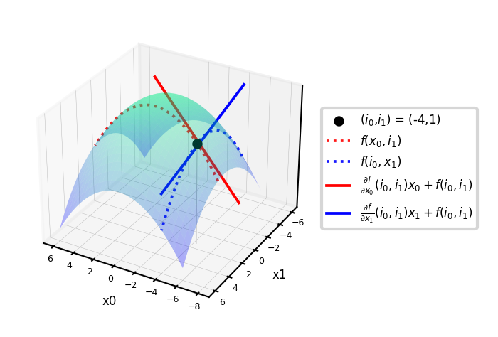
Example: \(f = -(x_0^2+x_1^2)\)
\(\nabla f = \left[\frac{\partial f}{\partial x_0},\frac{\partial f}{\partial x_1}\right] = \left[-2x_0,-2x_1\right]\)
Evaluated at point (-4,1): \(\nabla f(-4,1) = [8,-2]\)
These are the slopes at point (-4,1) in the direction of \(x_0\) and \(x_1\) respectively
Show code cell source
from mpl_toolkits import mplot3d
import ipywidgets as widgets
from ipywidgets import interact, interact_manual

# f = -(x0^2 + x1^2)
def g_f(x0, x1):
    return -(x0 ** 2 + x1 ** 2)
def g_dfx0(x0):
    return -2 * x0
def g_dfx1(x1):
    return -2 * x1

@interact
def plot_gradient(rotation=(0,240,10)):
    # plot surface of f
    fig = plt.figure(figsize=(12*fig_scale,5*fig_scale))
    ax = plt.axes(projection="3d")
    x0 = np.linspace(-6, 6, 30)
    x1 = np.linspace(-6, 6, 30)
    X0, X1 = np.meshgrid(x0, x1)
    ax.plot_surface(X0, X1, g_f(X0, X1), rstride=1, cstride=1,
                    cmap='winter', edgecolor='none',alpha=0.3)

    # choose point to evaluate: (-4,1)
    i0 = -4
    i1 = 1
    iz = np.linspace(g_f(i0,i1), -82, 30)
    ax.scatter3D(i0, i1, g_f(i0,i1), c="k", s=20*fig_scale,label='($i_0$,$i_1$) = (-4,1)')
    ax.plot3D([i0]*30, [i1]*30, iz, linewidth=1*fig_scale, c='silver', linestyle='-')
    ax.set_zlim(-80,0)

    # plot intersects
    ax.plot3D(x0,[1]*30,g_f(x0, 1),linewidth=3*fig_scale,alpha=0.9,label='$f(x_0,i_1)$',c='r',linestyle=':')
    ax.plot3D([-4]*30,x1,g_f(-4, x1),linewidth=3*fig_scale,alpha=0.9,label='$f(i_0,x_1)$',c='b',linestyle=':')

    # df/dx0 is slope of line at the intersect point
    x0 = np.linspace(-8, 0, 30)
    ax.plot3D(x0,[1]*30,g_dfx0(i0)*x0-g_f(i0,i1),linewidth=3*fig_scale,label=r'$\frac{\partial f}{\partial x_0}(i_0,i_1) x_0 + f(i_0,i_1)$',c='r',linestyle='-')
    ax.plot3D([-4]*30,x1,g_dfx1(i1)*x1+g_f(i0,i1),linewidth=3*fig_scale,label=r'$\frac{\partial f}{\partial x_1}(i_0,i_1) x_1 + f(i_0,i_1)$',c='b',linestyle='-')

    ax.set_xlabel('x0', labelpad=-4/fig_scale)
    ax.set_ylabel('x1', labelpad=-4/fig_scale)
    ax.get_zaxis().set_ticks([])
    ax.view_init(30, rotation) # Use this to rotate the figure
    ax.legend()
    box = ax.get_position()
    ax.set_position([box.x0, box.y0, box.width * 0.8, box.height])
    ax.legend(loc='center left', bbox_to_anchor=(1, 0.5))
    ax.tick_params(axis='both', width=0, labelsize=10*fig_scale, pad=-6)

    plt.tight_layout()
    plt.show()
Show code cell source
if not interactive:
    plot_gradient(rotation=120)
Distributions and Probabilities#
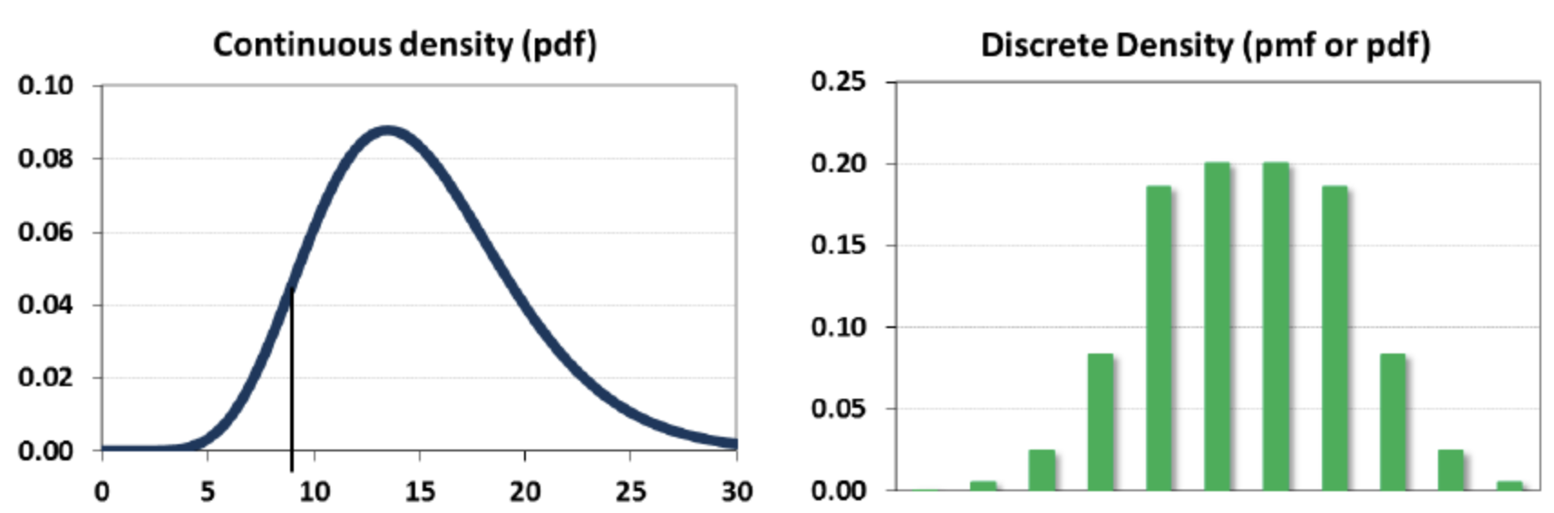
The normal (Gaussian) distribution with mean \(\mu\) and standard deviation \(\sigma\) is noted as \(N(\mu,\sigma)\)
A random variable \(X\) can be continuous or discrete
A probability distribution \(f_X\) of a continuous variable \(X\): probability density function (pdf)
The expectation is given by \(\mathbb{E}[X] = \int x f_{X}(x) dx\)
A probability distribution of a discrete variable: probability mass function (pmf)
The expectation (or mean) \(\mu_X = \mathbb{E}[X] = \sum_{i=1}^k[x_i \cdot Pr(X=x_i)]\)
Linear models#
Linear models make a prediction using a linear function of the input features \(X\)
Learn \(w\) from \(X\), given a loss function \(\mathcal{L}\):
Many algorithms with different \(\mathcal{L}\): Least squares, Ridge, Lasso, Logistic Regression, Linear SVMs,…
Can be very powerful (and fast), especially for large datasets with many features.
Can be generalized to learn non-linear patterns: Generalized Linear Models
Features can be augmentented with polynomials of the original features
Features can be transformed according to a distribution (Poisson, Tweedie, Gamma,…)
Some linear models (e.g. SVMs) can be kernelized to learn non-linear functions
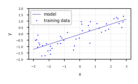
Linear models for regression#
Prediction formula for input features x:
\(w_1\) … \(w_p\) usually called weights or coefficients , \(w_0\) the bias or intercept
Assumes that errors are \(N(0,\sigma)\)
Show code cell source
from sklearn.linear_model import LinearRegression
from sklearn.model_selection import train_test_split
from mglearn.datasets import make_wave

Xw, yw = make_wave(n_samples=60)
Xw_train, Xw_test, yw_train, yw_test = train_test_split(Xw, yw, random_state=42)

line = np.linspace(-3, 3, 100).reshape(-1, 1)

lr = LinearRegression().fit(Xw_train, yw_train)
print("w_1: %f  w_0: %f" % (lr.coef_[0], lr.intercept_))

plt.figure(figsize=(6*fig_scale, 3*fig_scale))
plt.plot(line, lr.predict(line), lw=fig_scale)
plt.plot(Xw_train, yw_train, 'o', c='b')
#plt.plot(X_test, y_test, '.', c='r')
ax = plt.gca()
ax.grid(True)
ax.set_ylim(-2, 2)
ax.set_xlabel('x')
ax.set_ylabel('y')
ax.legend(["model", "training data"], loc="best");
w_1: 0.393906 w_0: -0.031804
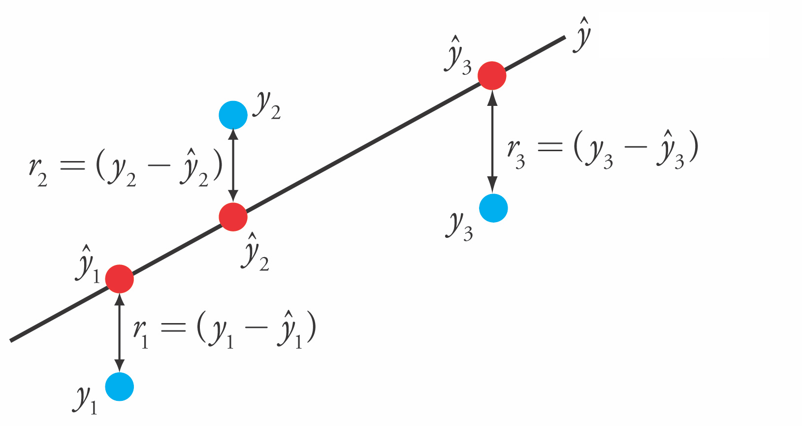
Linear Regression (aka Ordinary Least Squares)#
Loss function is the sum of squared errors (SSE) (or residuals) between predictions \(\hat{y}_i\) (red) and the true regression targets \(y_i\) (blue) on the training set.
Solving ordinary least squares#
Convex optimization problem with unique closed-form solution:
\[w^{*} = (X^{T}X)^{-1} X^T Y\]Add a column of 1’s to the front of X to get \(w_0\)
Slow. Time complexity is quadratic in number of features: \(\mathcal{O}(p^2n)\)
X has \(n\) rows, \(p\) features, hence \(X^{T}X\) has dimensionality \(p \cdot p\)
Only works if \(n>p\)
Gradient Descent
Faster for large and/or high-dimensional datasets
When \(X^{T}X\) cannot be computed or takes too long (\(p\) or \(n\) is too large)
When you want more control over the learning process
Very easily overfits.
coefficients \(w\) become very large (steep incline/decline)
small change in the input x results in a very different output y
No hyperparameters that control model complexity
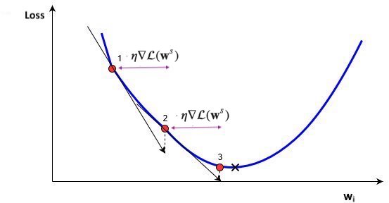
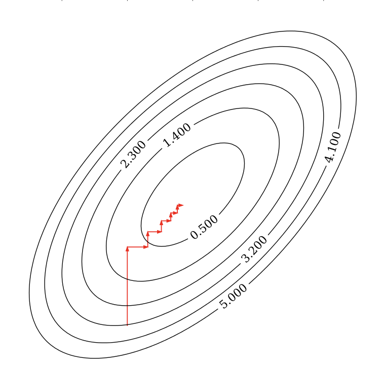
Gradient Descent#
Start with an initial, random set of weights: \(\mathbf{w}^0\)
Given a differentiable loss function \(\mathcal{L}\) (e.g. \(\mathcal{L}_{SSE}\)), compute \(\nabla \mathcal{L}\)
For least squares: \(\frac{\partial \mathcal{L}_{SSE}}{\partial w_i}(\mathbf{w}) = -2\sum_{n=1}^{N} (y_n-\hat{y}_n) x_{n,i}\)
If feature \(X_{:,i}\) is associated with big errors, the gradient wrt \(w_i\) will be large
Update all weights slightly (by step size or learning rate \(\eta\)) in ‘downhill’ direction.
Basic update rule (step s):
\[\mathbf{w}^{s+1} = \mathbf{w}^s-\eta\nabla \mathcal{L}(\mathbf{w}^s)\]
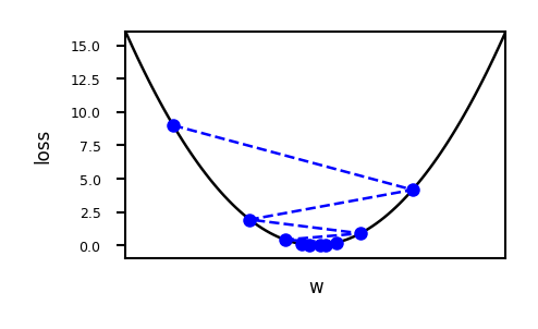
Important hyperparameters
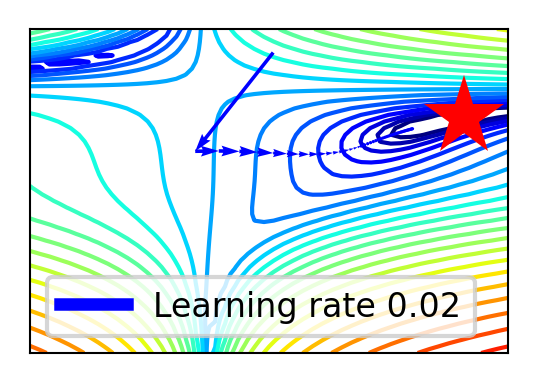
Learning rate
Too small: slow convergence. Too large: possible divergence
Maximum number of iterations
Too small: no convergence. Too large: wastes resources
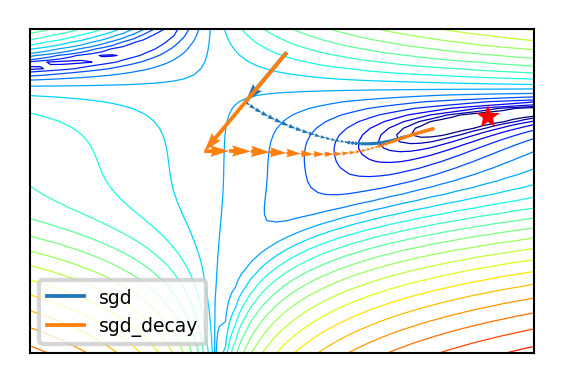
Learning rate decay with decay rate \(k\)
E.g. exponential (\(\eta^{s+1} = \eta^{0} e^{-ks}\)), inverse-time (\(\eta^{s+1} = \frac{\eta^{s}}{1+ks}\)),…
Many more advanced ways to control learning rate (see later)
Adaptive techniques: depend on how much loss improved in previous step
Show code cell source
import math
# Some convex function to represent the loss
def l_fx(x):
    return (x * 4)**2
# Derivative to compute the gradient
def l_dfx0(x0):
    return 8 * x0

@interact
def plot_learning_rate(learn_rate=(0.01,0.4,0.01), exp_decay=False):
    w = np.linspace(-1,1,101)
    f = [l_fx(i) for i in w]
    w_current = -0.75
    learn_rate_current = learn_rate
    fw = [] # weight values
    fl = [] # loss values
    for i in range(10):
        fw.append(w_current)
        fl.append(l_fx(w_current))
        # Decay
        if exp_decay:
            learn_rate_current = learn_rate * math.exp(-0.3*i)
        # Update rule
        w_current = w_current - learn_rate_current * l_dfx0(w_current)
    fig, ax = plt.subplots(figsize=(5*fig_scale,3*fig_scale))
    ax.set_xlabel('w')
    ax.set_xticks([])
    ax.set_ylabel('loss')
    ax.plot(w, f, lw=2*fig_scale, ls='-', c='k', label='Loss')
    ax.plot(fw, fl, '--bo', lw=2*fig_scale, markersize=3)
    plt.ylim(-1,16)
    plt.xlim(-1,1)
    plt.show()
Show code cell source
if not interactive:
    plot_learning_rate(learn_rate=0.21, exp_decay=False)
import tensorflow as tf
import numpy as np
import matplotlib.pyplot as plt

# Toy surface
def f(x, y):
    return (1.5 - x + x*y)**2 + (2.25 - x + x*y**2)**2 + (2.625 - x + x*y**3)**2

# TensorFlow optimizers
sgd = tf.optimizers.SGD(learning_rate=0.01)
lr_schedule = tf.optimizers.schedules.ExponentialDecay(
    initial_learning_rate=0.02,
    decay_steps=100,
    decay_rate=0.96
)
sgd_decay = tf.optimizers.SGD(learning_rate=lr_schedule)

optimizers = [sgd, sgd_decay]
opt_names = ['sgd', 'sgd_decay']
cmap = plt.cm.get_cmap('tab10')
colors = [cmap(x/10) for x in range(10)]

# Training
all_paths = []
for opt, name in zip(optimizers, opt_names):
    x = tf.Variable(0.8, dtype=tf.float32)
    y = tf.Variable(1.6, dtype=tf.float32)

    x_history = []
    y_history = []
    loss_prev = 0.0
    max_steps = 100

    for step in range(max_steps):
        with tf.GradientTape() as g:
            loss = f(x, y)

        x_history.append(x.numpy())
        y_history.append(y.numpy())
        grads = g.gradient(loss, [x, y])
        opt.apply_gradients(zip(grads, [x, y]))

        if np.abs(loss_prev - loss.numpy()) < 1e-6:
            break
        loss_prev = loss.numpy()

    x_history = np.array(x_history)
    y_history = np.array(y_history)
    path = np.vstack((x_history, y_history))
    all_paths.append(path)
Show code cell source
from matplotlib.colors import LogNorm

# Toy surface
def f(x, y):
    return (1.5 - x + x*y)**2 + (2.25 - x + x*y**2)**2 + (2.625 - x + x*y**3)**2

# Tensorflow optimizers
sgd = tf.optimizers.SGD(0.01)
lr_schedule = tf.optimizers.schedules.ExponentialDecay(0.02,decay_steps=100,decay_rate=0.96)
sgd_decay = tf.optimizers.SGD(learning_rate=lr_schedule)

optimizers = [sgd, sgd_decay]
opt_names = ['sgd', 'sgd_decay']
cmap = plt.cm.get_cmap('tab10')
colors = [cmap(x/10) for x in range(10)]

# Training
all_paths = []
for opt, name in zip(optimizers, opt_names):
    x_init = 0.8
    x = tf.Variable(x_init)
    y_init = 1.6
    y = tf.Variable(y_init)

    x_history = []
    y_history = []
    z_prev = 0.0
    max_steps = 100
    for step in range(max_steps):
        with tf.GradientTape() as g:
            z = f(x, y)
            x_history.append(x.numpy())
            y_history.append(y.numpy())
            dz_dx, dz_dy = g.gradient(z, [x, y])
            opt.apply_gradients(zip([dz_dx, dz_dy], [x, y]))

    if np.abs(z_prev - z.numpy()) < 1e-6:
        break
    z_prev = z.numpy()
    x_history = np.array(x_history)
    y_history = np.array(y_history)
    path = np.concatenate((np.expand_dims(x_history, 1), np.expand_dims(y_history, 1)), axis=1).T
    all_paths.append(path)

# Plotting
number_of_points = 50
margin = 4.5
minima = np.array([3., .5])
minima_ = minima.reshape(-1, 1)
x_min = 0. - 2
x_max = 0. + 3.5
y_min = 0. - 3.5
y_max = 0. + 2
x_points = np.linspace(x_min, x_max, number_of_points)
y_points = np.linspace(y_min, y_max, number_of_points)
x_mesh, y_mesh = np.meshgrid(x_points, y_points)
z = np.array([f(xps, yps) for xps, yps in zip(x_mesh, y_mesh)])

def plot_optimizers(ax, iterations, optimizers):
    ax.contour(x_mesh, y_mesh, z, levels=np.logspace(-0.5, 5, 25), norm=LogNorm(), cmap=plt.cm.jet, linewidths=fig_scale, zorder=-1)
    ax.plot(*minima, 'r*', markersize=20*fig_scale)
    for name, path, color in zip(opt_names, all_paths, colors):
        if name in optimizers:
            p = path[:,:iterations]
            ax.plot([], [], color=color, label=name, lw=3*fig_scale, linestyle='-')
            ax.quiver(p[0,:-1], p[1,:-1], p[0,1:]-p[0,:-1], p[1,1:]-p[1,:-1], scale_units='xy', angles='xy', scale=1, color=color, lw=4)


    ax.set_xlim((x_min, x_max))
    ax.set_ylim((y_min, y_max))
    ax.legend(loc='lower left', prop={'size': 15*fig_scale})
    ax.set_xticks([])
    ax.set_yticks([])
    plt.tight_layout()
# Training for momentum
all_lr_paths = []
lr_range = [0.005 * i for i in range(10)]

for lr in lr_range:
    opt = tf.optimizers.SGD(learning_rate=lr, nesterov=False)

    x = tf.Variable(0.8, dtype=tf.float32)
    y = tf.Variable(1.6, dtype=tf.float32)

    x_history = []
    y_history = []
    z_prev = 0.0
    max_steps = 100

    for step in range(max_steps):
        with tf.GradientTape() as g:
            z = f(x, y)

        x_history.append(x.numpy())
        y_history.append(y.numpy())
        dz_dx, dz_dy = g.gradient(z, [x, y])
        opt.apply_gradients(zip([dz_dx, dz_dy], [x, y]))

        if np.abs(z_prev - z.numpy()) < 1e-6:
            break
        z_prev = z.numpy()

    x_history = np.array(x_history)
    y_history = np.array(y_history)
    path = np.vstack((x_history, y_history))
    all_lr_paths.append(path)

# Plotting
number_of_points = 50
margin = 4.5
minima = np.array([3., 0.5])
minima_ = minima.reshape(-1, 1)
x_min = -2
x_max = 3.5
y_min = -3.5
y_max = 2
x_points = np.linspace(x_min, x_max, number_of_points)
y_points = np.linspace(y_min, y_max, number_of_points)
x_mesh, y_mesh = np.meshgrid(x_points, y_points)
z = np.array([[f(xps, yps) for xps, yps in zip(row_x, row_y)] for row_x, row_y in zip(x_mesh, y_mesh)])

def plot_learning_rate_optimizers(ax, iterations, lr):
    ax.contour(x_mesh, y_mesh, z, levels=np.logspace(-0.5, 5, 25), norm=LogNorm(), cmap=plt.cm.jet, linewidths=1, zorder=-1)
    ax.plot(*minima, 'r*', markersize=20)

    for path, lrate in zip(all_lr_paths, lr_range):
        if round(lrate, 3) == round(lr, 3):
            p = path[:, :iterations]
            ax.plot([], [], color='b', label=f"Learning rate {round(lr, 3)}", lw=3, linestyle='-')
            ax.quiver(p[0, :-1], p[1, :-1], p[0, 1:] - p[0, :-1], p[1, 1:] - p[1, :-1], scale_units='xy', angles='xy', scale=1, color='b', lw=4)

    ax.set_xlim((x_min, x_max))
    ax.set_ylim((y_min, y_max))
    ax.legend(loc='lower left', prop={'size': 8})
    ax.set_xticks([])
    ax.set_yticks([])
    plt.tight_layout()
Effect of learning rate
Show code cell source
@interact
def plot_lr(iterations=(1, 100, 1), learning_rate=(0.005, 0.045, 0.005)):  # Fixed range
    fig, ax = plt.subplots(figsize=(6 * fig_scale, 4 * fig_scale))
    plot_learning_rate_optimizers(ax, iterations, learning_rate)
    plt.show()

if not interactive:
    plot_lr(iterations=50, learning_rate=0.02)
Effect of learning rate decay
Show code cell source
@interact
def compare_optimizers(iterations=(1,100,1), optimizer1=opt_names, optimizer2=opt_names):
    fig, ax = plt.subplots(figsize=(6*fig_scale,4*fig_scale))
    plot_optimizers(ax,iterations,[optimizer1,optimizer2])
    plt.show()

if not interactive:
    compare_optimizers(iterations=50, optimizer1="sgd", optimizer2="sgd_decay")
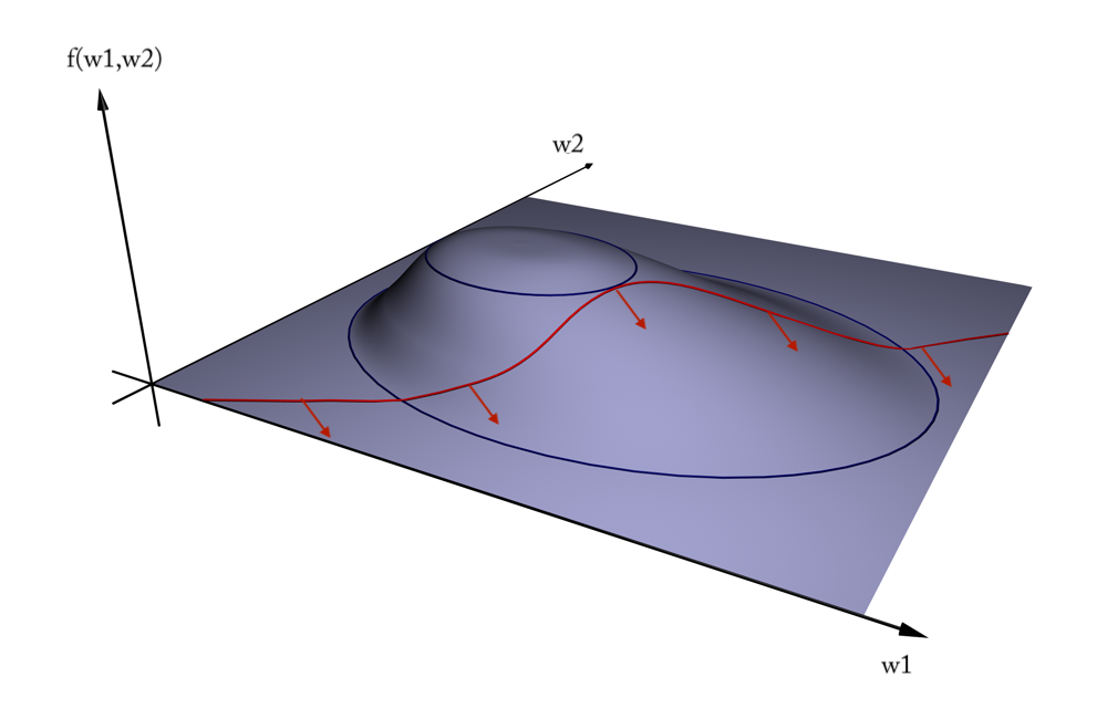
In two dimensions:
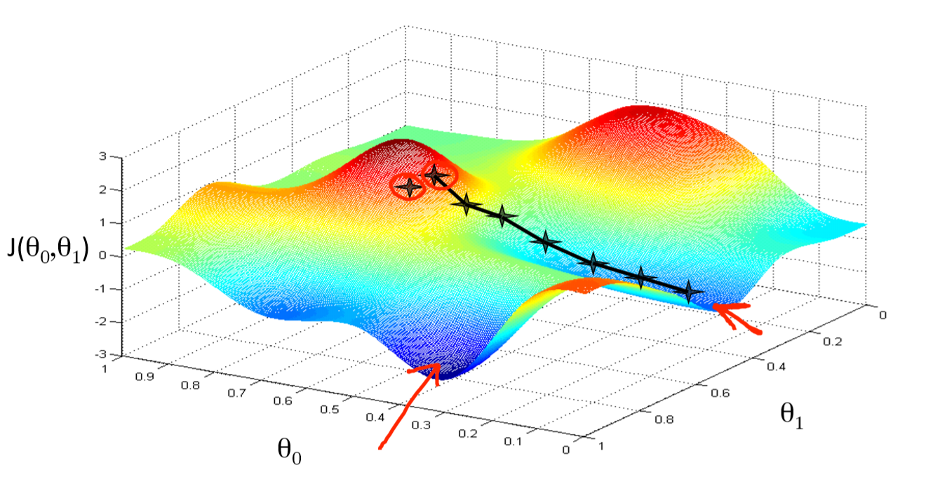
You can get stuck in local minima (if the loss is not fully convex)
If you have many model parameters, this is less likely
You always find a way down in some direction
Models with many parameters typically find good local minima
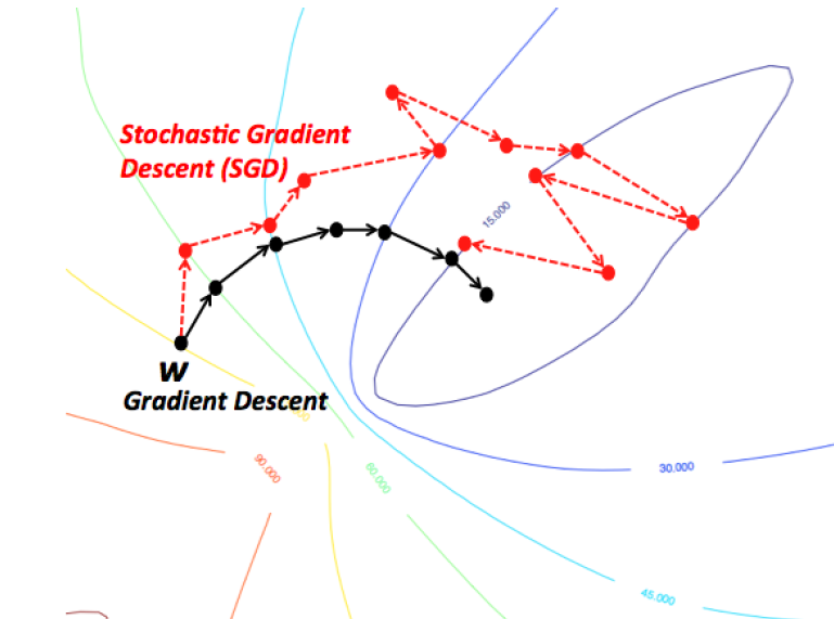
Intuition: walking downhill using only the slope you “feel” nearby
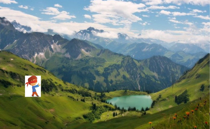
(Image by A. Karpathy)
Stochastic Gradient Descent (SGD)#
Compute gradients not on the entire dataset, but on a single data point \(i\) at a time
Gradient descent: \(\mathbf{w}^{s+1} = \mathbf{w}^s-\eta\nabla \mathcal{L}(\mathbf{w}^s) = \mathbf{w}^s-\frac{\eta}{n} \sum_{i=1}^{n} \nabla \mathcal{L_i}(\mathbf{w}^s)\)
Stochastic Gradient Descent: \(\mathbf{w}^{s+1} = \mathbf{w}^s-\eta\nabla \mathcal{L_i}(\mathbf{w}^s)\)
Many smoother variants, e.g.
Minibatch SGD: compute gradient on batches of data: \(\mathbf{w}^{s+1} = \mathbf{w}^s-\frac{\eta}{B} \sum_{i=1}^{B} \nabla \mathcal{L_i}(\mathbf{w}^s)\)
Stochastic Average Gradient Descent (SAG, SAGA). With \(i_s \in [1,n]\) randomly chosen per iteration:
Incremental gradient: \(\mathbf{w}^{s+1} = \mathbf{w}^s-\frac{\eta}{n} \sum_{i=1}^{n} v_i^s\) with \(v_i^s = \begin{cases}\nabla \mathcal{L_i}(\mathbf{w}^s) & i = i_s \\ v_i^{s-1} & \text{otherwise} \end{cases}\)
In practice#
Linear regression can be found in
sklearn.linear_model. We’ll evaluate it on the Boston Housing dataset.LinearRegressionuses closed form solution,SGDRegressorwithloss='squared_loss'uses Stochastic Gradient DescentLarge coefficients signal overfitting
Test score is much lower than training score
from sklearn.linear_model import LinearRegression
lr = LinearRegression().fit(X_train, y_train)
Show code cell source
from sklearn.model_selection import train_test_split
from sklearn.linear_model import LinearRegression

X_B, y_B = mglearn.datasets.load_extended_boston()
X_B_train, X_B_test, y_B_train, y_B_test = train_test_split(X_B, y_B, random_state=0)

lr = LinearRegression().fit(X_B_train, y_B_train)
Show code cell source
print("Weights (coefficients): {}".format(lr.coef_[0:40]))
print("Bias (intercept): {}".format(lr.intercept_))
Weights (coefficients): [ -412.711   -52.243  -131.899   -12.004   -15.511    28.716    54.704
   -49.535    26.582    37.062   -11.828   -18.058   -19.525    12.203
  2980.781  1500.843   114.187   -16.97     40.961   -24.264    57.616
  1278.121 -2239.869   222.825    -2.182    42.996   -13.398   -19.389
    -2.575   -81.013     9.66      4.914    -0.812    -7.647    33.784
   -11.446    68.508   -17.375    42.813     1.14 ]
Bias (intercept): 30.93456367364179
Show code cell source
print("Training set score (R^2): {:.2f}".format(lr.score(X_B_train, y_B_train)))
print("Test set score (R^2): {:.2f}".format(lr.score(X_B_test, y_B_test)))
Training set score (R^2): 0.95
Test set score (R^2): 0.61
Ridge regression#
Adds a penalty term to the least squares loss function:
Model is penalized if it uses large coefficients (\(w\))
Each feature should have as little effect on the outcome as possible
We don’t want to penalize \(w_0\), so we leave it out
Regularization: explicitly restrict a model to avoid overfitting.
Called L2 regularization because it uses the L2 norm: \(\sum w_i^2\)
The strength of the regularization can be controlled with the \(\alpha\) hyperparameter.
Increasing \(\alpha\) causes more regularization (or shrinkage). Default is 1.0.
Still convex. Can be optimized in different ways:
Closed form solution (a.k.a. Cholesky): \(w^{*} = (X^{T}X + \alpha I)^{-1} X^T Y\)
Gradient descent and variants, e.g. Stochastic Average Gradient (SAG,SAGA)
Conjugate gradient (CG): each new gradient is influenced by previous ones
Use Cholesky for smaller datasets, Gradient descent for larger ones
In practice#
from sklearn.linear_model import Ridge
lr = Ridge().fit(X_train, y_train)
Show code cell source
from sklearn.linear_model import Ridge
ridge = Ridge().fit(X_B_train, y_B_train)
print("Weights (coefficients): {}".format(ridge.coef_[0:40]))
print("Bias (intercept): {}".format(ridge.intercept_))
print("Training set score: {:.2f}".format(ridge.score(X_B_train, y_B_train)))
print("Test set score: {:.2f}".format(ridge.score(X_B_test, y_B_test)))
Weights (coefficients): [-1.414 -1.557 -1.465 -0.127 -0.079  8.332  0.255 -4.941  3.899 -1.059
 -1.584  1.051 -4.012  0.334  0.004 -0.849  0.745 -1.431 -1.63  -1.405
 -0.045 -1.746 -1.467 -1.332 -1.692 -0.506  2.622 -2.092  0.195 -0.275
  5.113 -1.671 -0.098  0.634 -0.61   0.04  -1.277 -2.913  3.395  0.792]
Bias (intercept): 21.39052595861006
Training set score: 0.89
Test set score: 0.75
Test set score is higher and training set score lower: less overfitting!
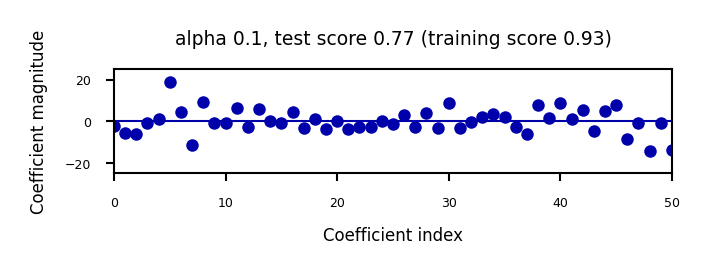
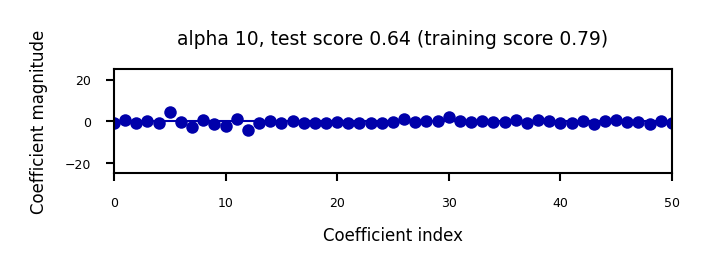
We can plot the weight values for differents levels of regularization to explore the effect of \(\alpha\).
Increasing regularization decreases the values of the coefficients, but never to 0.
Show code cell source
from __future__ import print_function
import ipywidgets as widgets
from ipywidgets import interact, interact_manual
from sklearn.linear_model import Ridge

@interact
def plot_ridge(alpha=(0,10.0,0.05)):
    r = Ridge(alpha=alpha).fit(X_B_train, y_B_train)
    fig, ax = plt.subplots(figsize=(8*fig_scale,1.5*fig_scale))
    ax.plot(r.coef_, 'o', markersize=3)
    ax.set_title("alpha {}, test score {:.2f} (training score {:.2f})".format(alpha, r.score(X_B_test, y_B_test), r.score(X_B_train, y_B_train)))
    ax.set_xlabel("Coefficient index")
    ax.set_ylabel("Coefficient magnitude")
    ax.hlines(0, 0, len(r.coef_))
    ax.set_ylim(-25, 25)
    ax.set_xlim(0, 50);
    plt.show()
Show code cell source
if not interactive:
    for alpha in [0.1, 10]:
        plot_ridge(alpha)
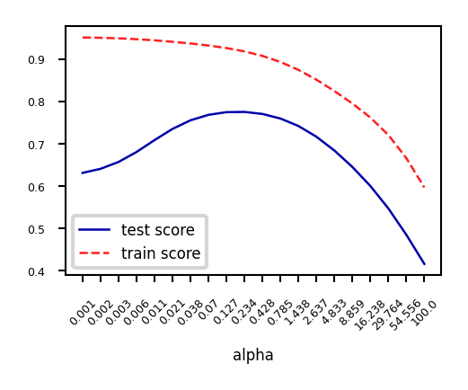
When we plot the train and test scores for every \(\alpha\) value, we see a sweet spot around \(\alpha=0.2\)
Models with smaller \(\alpha\) are overfitting
Models with larger \(\alpha\) are underfitting
Show code cell source
alpha=np.logspace(-3,2,num=20)
ai = list(range(len(alpha)))
test_score=[]
train_score=[]
for a in alpha:
    r = Ridge(alpha=a).fit(X_B_train, y_B_train)
    test_score.append(r.score(X_B_test, y_B_test))
    train_score.append(r.score(X_B_train, y_B_train))
fig, ax = plt.subplots(figsize=(6*fig_scale,4*fig_scale))
ax.set_xticks(range(20))
ax.set_xticklabels(np.round(alpha,3))
ax.set_xlabel('alpha')
ax.plot(test_score, lw=2*fig_scale, label='test score')
ax.plot(train_score, lw=2*fig_scale, label='train score')
ax.legend()
plt.xticks(rotation=45);
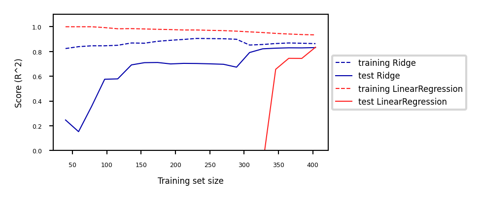
Other ways to reduce overfitting#
Add more training data: with enough training data, regularization becomes less important
Ridge and ordinary least squares will have the same performance
Use fewer features: remove unimportant ones or find a low-dimensional embedding (e.g. PCA)
Fewer coefficients to learn, reduces the flexibility of the model
Scaling the data typically helps (and changes the optimal \(\alpha\) value)
Show code cell source
fig, ax = plt.subplots(figsize=(10*fig_scale,4*fig_scale))
mglearn.plots.plot_ridge_n_samples(ax)
Lasso (Least Absolute Shrinkage and Selection Operator)#
Adds a different penalty term to the least squares sum:
Called L1 regularization because it uses the L1 norm
Will cause many weights to be exactly 0
Same parameter \(\alpha\) to control the strength of regularization.
Will again have a ‘sweet spot’ depending on the data
No closed-form solution
Convex, but no longer strictly convex, and not differentiable
Weights can be optimized using coordinate descent
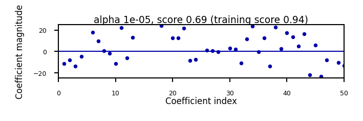
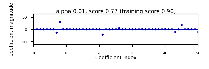
Analyze what happens to the weights:
L1 prefers coefficients to be exactly zero (sparse models)
Some features are ignored entirely: automatic feature selection
How can we explain this?
Show code cell source
from sklearn.linear_model import Lasso

@interact
def plot_lasso(alpha=(0,0.5,0.005)):
    r = Lasso(alpha=alpha).fit(X_B_train, y_B_train)
    fig, ax = plt.subplots(figsize=(8*fig_scale,1.5*fig_scale))
    ax.plot(r.coef_, 'o', markersize=6*fig_scale)
    ax.set_title("alpha {}, score {:.2f} (training score {:.2f})".format(alpha, r.score(X_B_test, y_B_test), r.score(X_B_train, y_B_train)), pad=0.5)
    ax.set_xlabel("Coefficient index", labelpad=0)
    ax.set_ylabel("Coefficient magnitude")
    ax.hlines(0, 0, len(r.coef_))
    ax.set_ylim(-25, 25);
    ax.set_xlim(0, 50);
    plt.show()
Show code cell source
if not interactive:
    for alpha in [0.00001, 0.01]:
        plot_lasso(alpha)
Coordinate descent#
Alternative for gradient descent, supports non-differentiable convex loss functions (e.g. \(\mathcal{L}_{Lasso}\))
In every iteration, optimize a single coordinate \(w_i\) (find minimum in direction of \(x_i\))
Continue with another coordinate, using a selection rule (e.g. round robin)
Faster iterations. No need to choose a step size (learning rate).
May converge more slowly. Can’t be parallellized.
Coordinate descent with Lasso#
Remember that \(\mathcal{L}_{Lasso} = \mathcal{L}_{SSE} + \alpha \sum_{i=1}^{p} |w_i|\)
For one \(w_i\): \(\mathcal{L}_{Lasso}(w_i) = \mathcal{L}_{SSE}(w_i) + \alpha |w_i|\)
The L1 term is not differentiable but convex: we can compute the subgradient
Unique at points where \(\mathcal{L}\) is differentiable, a range of all possible slopes [a,b] where it is not
For \(|w_i|\), the subgradient \(\partial_{w_i} |w_i|\) = \(\begin{cases}-1 & w_i<0\\ [-1,1] & w_i=0 \\ 1 & w_i>0 \\ \end{cases}\)
Subdifferential \(\partial(f+g) = \partial f + \partial g\) if \(f\) and \(g\) are both convex
To find the optimum for Lasso \(w_i^{*}\), solve
\[\begin{split}\begin{aligned} \partial_{w_i} \mathcal{L}_{Lasso}(w_i) &= \partial_{w_i} \mathcal{L}_{SSE}(w_i) + \partial_{w_i} \alpha |w_i| \\ 0 &= (w_i - \rho_i) + \alpha \cdot \partial_{w_i} |w_i| \\ w_i &= \rho_i - \alpha \cdot \partial_{w_i} |w_i| \end{aligned}\end{split}\]In which \(\rho_i\) is the part of \(\partial_{w_i} \mathcal{L}_{SSE}(w_i)\) excluding \(w_i\) (assume \(z_i=1\) for now)
\(\rho_i\) can be seen as the \(\mathcal{L}_{SSE}\) ‘solution’: \(w_i = \rho_i\) if \(\partial_{w_i} \mathcal{L}_{SSE}(w_i) = 0\) $\(\partial_{w_i} \mathcal{L}_{SSE}(w_i) = \partial_{w_i} \sum_{n=1}^{N} (y_n-(\mathbf{w}\mathbf{x_n} + w_0))^2 = z_i w_i -\rho_i \)$
We found: \(w_i = \rho_i - \alpha \cdot \partial_{w_i} |w_i|\)
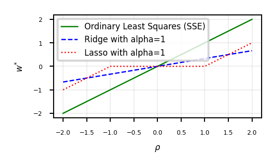
The Lasso solution has the form of a soft thresholding function \(S\)
\[\begin{split}w_i^* = S(\rho_i,\alpha) = \begin{cases} \rho_i + \alpha, & \rho_i < -\alpha \\ 0, & -\alpha < \rho_i < \alpha \\ \rho_i - \alpha, & \rho_i > \alpha \\ \end{cases}\end{split}\]Small weights (all weights between \(-\alpha\) and \(\alpha\)) become 0: sparseness!
If the data is not normalized, \(w_i^* = \frac{1}{z_i}S(\rho_i,\alpha)\) with constant \(z_i = \sum_{n=1}^{N} x_{ni}^2\)
Ridge solution: \(w_i = \rho_i - \alpha \cdot \partial_{w_i} w_i^2 = \rho_i - 2\alpha \cdot w_i\), thus \(w_i^* = \frac{\rho_i}{1 + 2\alpha}\)
Show code cell source
@interact
def plot_rho(alpha=(0,2.0,0.05)):
    w = np.linspace(-2,2,101)
    r = w/(1+2*alpha)
    l = [x+alpha if x <= -alpha else (x-alpha if x > alpha else 0) for x in w]
    fig, ax = plt.subplots(figsize=(6*fig_scale,3*fig_scale))
    ax.set_xlabel(r'$\rho$')
    ax.set_ylabel(r'$w^{*}$')
    ax.plot(w, w, lw=2*fig_scale, c='g', label='Ordinary Least Squares (SSE)')
    ax.plot(w, r, lw=2*fig_scale, c='b', label='Ridge with alpha={}'.format(alpha))
    ax.plot(w, l, lw=2*fig_scale, c='r', label='Lasso with alpha={}'.format(alpha))
    ax.legend()
    plt.grid()
    plt.show()
Show code cell source
if not interactive:
    plot_rho(alpha=1)
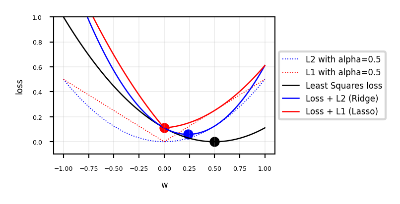
Interpreting L1 and L2 loss#
L1 and L2 in function of the weights
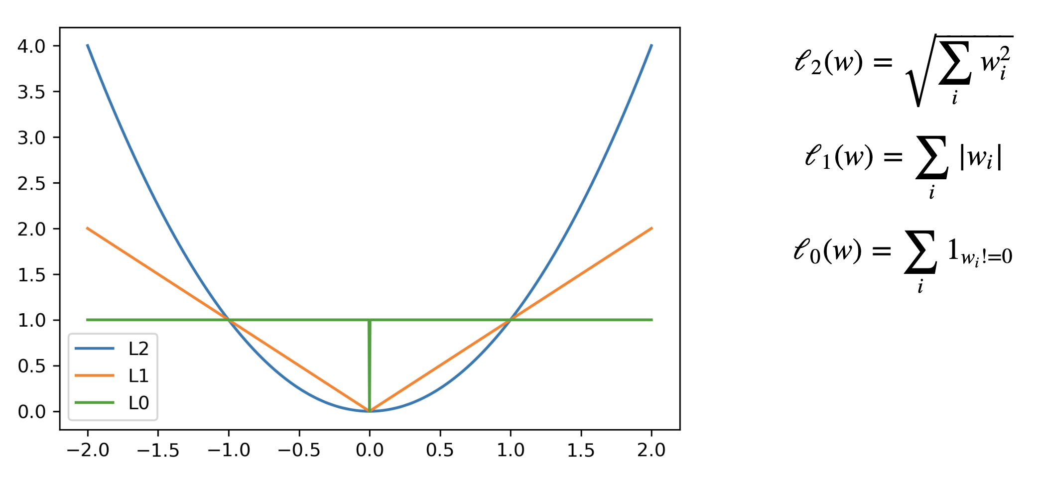
Least Squares Loss + L1 or L2
The Lasso curve has 3 parts (\(w<0\),\(w=0\),\(w>0\)) corresponding to the thresholding function
For any minimum of least squares, L2 will be smaller, and L1 is more likely be exactly 0
Show code cell source
def c_fx(x):
    fX = ((x * 2 - 1)**2) # Some convex function to represent the loss
    return fX/9 # Scaling
def c_fl2(x,alpha):
    return c_fx(x) + alpha * x**2
def c_fl1(x,alpha):
    return c_fx(x) + alpha * abs(x)
def l2(x,alpha):
    return alpha * x**2
def l1(x,alpha):
    return alpha * abs(x)

@interact
def plot_losses(alpha=(0,1.0,0.05)):
    w = np.linspace(-1,1,101)
    f = [c_fx(i) for i in w]
    r = [c_fl2(i,alpha) for i in w]
    l = [c_fl1(i,alpha) for i in w]
    rp = [l2(i,alpha) for i in w]
    lp = [l1(i,alpha) for i in w]
    fig, ax = plt.subplots(figsize=(8*fig_scale,4*fig_scale))
    ax.set_xlabel('w')
    ax.set_ylabel('loss')
    ax.plot(w, rp, lw=1.5*fig_scale, ls=':', c='b', label='L2 with alpha={}'.format(alpha))
    ax.plot(w, lp, lw=1.5*fig_scale, ls=':', c='r', label='L1 with alpha={}'.format(alpha))
    ax.plot(w, f, lw=2*fig_scale, ls='-', c='k', label='Least Squares loss')
    ax.plot(w, r, lw=2*fig_scale, ls='-', c='b', label='Loss + L2 (Ridge)'.format(alpha))
    ax.plot(w, l, lw=2*fig_scale, ls='-', c='r', label='Loss + L1 (Lasso)'.format(alpha))
    opt_f = np.argmin(f)
    ax.scatter(w[opt_f], f[opt_f], c="k", s=50*fig_scale)
    opt_r = np.argmin(r)
    ax.scatter(w[opt_r], r[opt_r], c="b", s=50*fig_scale)
    opt_l = np.argmin(l)
    ax.scatter(w[opt_l], l[opt_l], c="r", s=50*fig_scale)
    ax.legend()
    box = ax.get_position()
    ax.set_position([box.x0, box.y0, box.width * 0.8, box.height])
    ax.legend(loc='center left', bbox_to_anchor=(1, 0.5))
    plt.ylim(-0.1,1)
    plt.grid()
    plt.show()
Show code cell source
if not interactive:
    plot_losses(alpha=0.5)
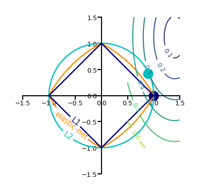
In 2D (for 2 model weights \(w_1\) and \(w_2\))
The least squared loss is a 2D convex function in this space (ellipses on the right)
For illustration, assume that L1 loss = L2 loss = 1
L1 loss (\(\Sigma |w_i|\)): the optimal {\(w_1, w_2\)} (blue dot) falls on the diamond
L2 loss (\(\Sigma w_i^2\)): the optimal {\(w_1, w_2\)} (cyan dot) falls on the circle
For L1, the loss is minimized if \(w_1\) or \(w_2\) is 0 (rarely so for L2)
Show code cell source
def plot_loss_interpretation():
    line = np.linspace(-1.5, 1.5, 1001)
    xx, yy = np.meshgrid(line, line)

    l2 = xx ** 2 + yy ** 2
    l1 = np.abs(xx) + np.abs(yy)
    rho = 0.7
    elastic_net = rho * l1 + (1 - rho) * l2

    plt.figure(figsize=(5*fig_scale, 4*fig_scale))
    ax = plt.gca()

    elastic_net_contour = plt.contour(xx, yy, elastic_net, levels=[1], linewidths=2*fig_scale, colors="darkorange")
    l2_contour = plt.contour(xx, yy, l2, levels=[1], linewidths=2*fig_scale, colors="c")
    l1_contour = plt.contour(xx, yy, l1, levels=[1], linewidths=2*fig_scale, colors="navy")
    ax.set_aspect("equal")
    ax.spines['left'].set_position('center')
    ax.spines['right'].set_color('none')
    ax.spines['bottom'].set_position('center')
    ax.spines['top'].set_color('none')

    plt.clabel(elastic_net_contour, inline=1, fontsize=12*fig_scale,
               fmt={1.0: 'elastic-net'}, manual=[(-0.6, -0.6)])
    plt.clabel(l2_contour, inline=1, fontsize=12*fig_scale,
               fmt={1.0: 'L2'}, manual=[(-0.5, -0.5)])
    plt.clabel(l1_contour, inline=1, fontsize=12*fig_scale,
               fmt={1.0: 'L1'}, manual=[(-0.5, -0.5)])

    x1 = np.linspace(0.5, 1.5, 100)
    x2 = np.linspace(-1.0, 1.5, 100)
    X1, X2 = np.meshgrid(x1, x2)
    Y = np.sqrt(np.square(X1/2-0.7) + np.square(X2/4-0.28))
    cp = plt.contour(X1, X2, Y)
    plt.clabel(cp, inline=1, fontsize=3)
    ax.tick_params(axis='both', pad=0)
    ax.scatter(1, 0, c="navy", s=50*fig_scale)
    ax.scatter(0.89, 0.42, c="c", s=50*fig_scale)

    plt.tight_layout()
    plt.show()
plot_loss_interpretation()
Elastic-Net#
Adds both L1 and L2 regularization:
\(\rho\) is the L1 ratio
With \(\rho=1\), \(\mathcal{L}_{Elastic} = \mathcal{L}_{Lasso}\)
With \(\rho=0\), \(\mathcal{L}_{Elastic} = \mathcal{L}_{Ridge}\)
\(0 < \rho < 1\) sets a trade-off between L1 and L2.
Allows learning sparse models (like Lasso) while maintaining L2 regularization benefits
E.g. if 2 features are correlated, Lasso likely picks one randomly, Elastic-Net keeps both
Weights can be optimized using coordinate descent (similar to Lasso)
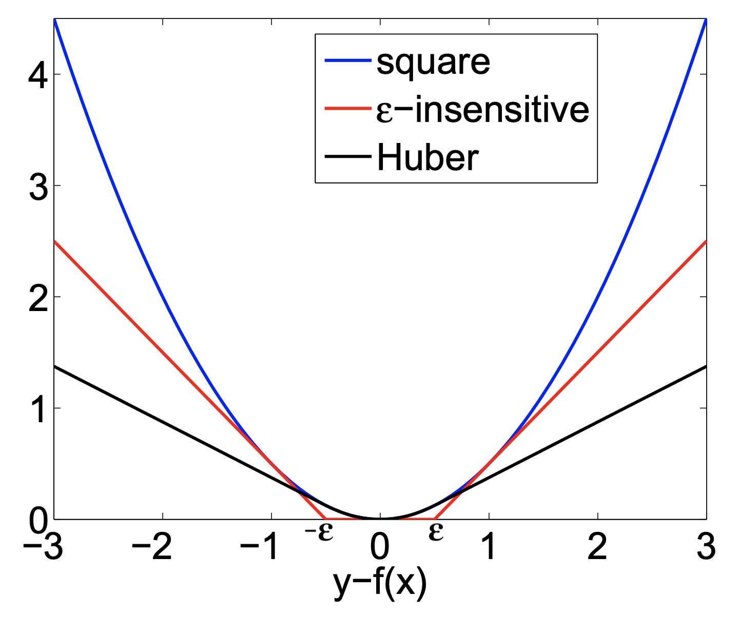
Other loss functions for regression#
Huber loss: switches from squared loss to linear loss past a value \(\epsilon\)
More robust against outliers
Epsilon insensitive: ignores errors smaller than \(\epsilon\), and linear past that
Aims to fit function so that residuals are at most \(\epsilon\)
Also known as Support Vector Regression (
SVRin sklearn)
Squared Epsilon insensitive: ignores errors smaller than \(\epsilon\), and squared past that
These can all be solved with stochastic gradient descent
SGDRegressorin sklearn
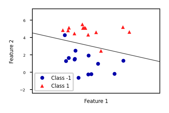
Linear models for Classification#
Aims to find a hyperplane that separates the examples of each class.
For binary classification (2 classes), we aim to fit the following function:
\(\hat{y} = w_1 * x_1 + w_2 * x_2 +... + w_p * x_p + w_0 > 0\)
When \(\hat{y}<0\), predict class -1, otherwise predict class +1
Show code cell source
from sklearn.linear_model import LogisticRegression
from sklearn.svm import LinearSVC

Xf, yf = mglearn.datasets.make_forge()
fig, ax = plt.subplots(figsize=(6*fig_scale,4*fig_scale))
clf = LogisticRegression().fit(Xf, yf)
mglearn.tools.plot_2d_separator(clf, Xf,
                                ax=ax, alpha=.7, cm=mglearn.cm2)
mglearn.discrete_scatter(Xf[:, 0], Xf[:, 1], yf, ax=ax, s=10*fig_scale)
ax.set_xlabel("Feature 1")
ax.set_ylabel("Feature 2")
ax.legend(['Class -1','Class 1']);
There are many algorithms for linear classification, differing in loss function, regularization techniques, and optimization method
Most common techniques:
Convert target classes {neg,pos} to {0,1} and treat as a regression task
Logistic regression (Log loss)
Ridge Classification (Least Squares + L2 loss)
Find hyperplane that maximizes the margin between classes
Linear Support Vector Machines (Hinge loss)
Neural networks without activation functions
Perceptron (Perceptron loss)
SGDClassifier: can act like any of these by choosing loss function
Hinge, Log, Modified_huber, Squared_hinge, Perceptron
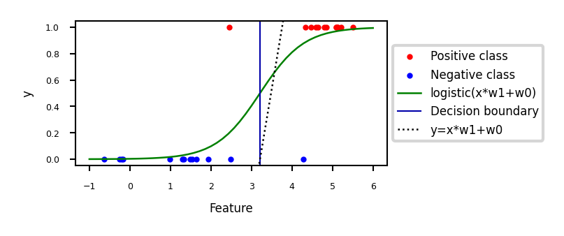
Logistic regression#
Aims to predict the probability that a point belongs to the positive class
Converts target values {negative (blue), positive (red)} to {0,1}
Fits a logistic (or sigmoid or S curve) function through these points
Maps (-Inf,Inf) to a probability [0,1]
\[ \hat{y} = \textrm{logistic}(f_{\theta}(\mathbf{x})) = \frac{1}{1+e^{-f_{\theta}(\mathbf{x})}} \]E.g. in 1D: \( \textrm{logistic}(x_1w_1+w_0) = \frac{1}{1+e^{-x_1w_1-w_0}} \)
Show code cell source
def sigmoid(x,w1,w0):
    return 1 / (1 + np.exp(-(x*w1+w0)))

@interact
def plot_logreg(w0=(-10.0,5.0,1),w1=(-1.0,3.0,0.3)):
    fig, ax = plt.subplots(figsize=(8*fig_scale,3*fig_scale))
    red = [Xf[i, 1] for i in range(len(yf)) if yf[i]==1]
    blue = [Xf[i, 1] for i in range(len(yf)) if yf[i]==0]
    ax.scatter(red, [1]*len(red), c='r', label='Positive class')
    ax.scatter(blue, [0]*len(blue), c='b', label='Negative class')
    x = np.linspace(min(-1, -w0/w1),max(6, -w0/w1))
    ax.plot(x,sigmoid(x,w1,w0),lw=2*fig_scale,c='g', label='logistic(x*w1+w0)'.format(np.round(w0,2),np.round(w1,2)))
    ax.axvline(x=(-w0/w1), ymin=0, ymax=1, label='Decision boundary')
    ax.plot(x,x*w1+w0,lw=2*fig_scale,c='k',linestyle=':', label='y=x*w1+w0')
    ax.set_xlabel("Feature")
    ax.set_ylabel("y")
    ax.set_ylim(-0.05,1.05)
    ax.legend(loc='center left', bbox_to_anchor=(1, 0.5))
    box = ax.get_position()
    ax.set_position([box.x0, box.y0, box.width * 0.8, box.height]);
    plt.show()
Show code cell source
if not interactive:
    # fitted solution
    clf2 = LogisticRegression(C=100).fit(Xf[:, 1].reshape(-1, 1), yf)
    w0 = clf2.intercept_
    w1 = clf2.coef_[0][0]
    plot_logreg(w0=w0,w1=w1)
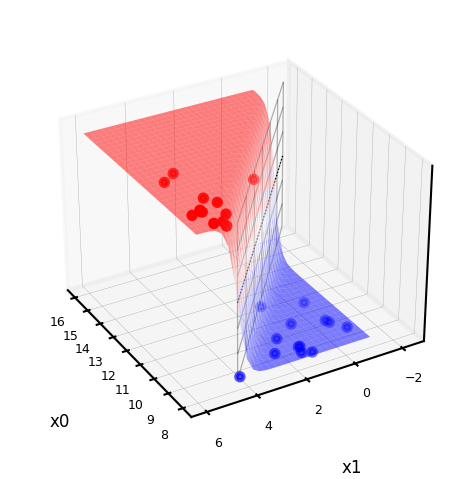
Fitted solution to our 2D example:
To get a binary prediction, choose a probability threshold (e.g. 0.5)
Show code cell source
lr_clf = LogisticRegression(C=100).fit(Xf, yf)

def sigmoid2d(x1,x2,w0,w1,w2):
    return 1 / (1 + np.exp(-(x2*w2+x1*w1+w0)))

@interact
def plot_logistic_fit(rotation=(0,360,10)):
    w0 = lr_clf.intercept_
    w1 = lr_clf.coef_[0][0]
    w2 = lr_clf.coef_[0][1]

    # plot surface of f
    fig = plt.figure(figsize=(7*fig_scale,5*fig_scale))
    ax = plt.axes(projection="3d")
    x0 = np.linspace(8, 16, 30)
    x1 = np.linspace(-1, 6, 30)
    X0, X1 = np.meshgrid(x0, x1)

    # Surface
    ax.plot_surface(X0, X1, sigmoid2d(X0, X1, w0, w1, w2), rstride=1, cstride=1,
                    cmap='bwr', edgecolor='none',alpha=0.5,label='sigmoid')
    # Points
    c=['b','r']
    ax.scatter3D(Xf[:, 0], Xf[:, 1], yf, c=[c[i] for i in yf], s=10*fig_scale)

    # Decision boundary
    # x2 = -(x1*w1 + w0)/w2
    ax.plot3D(x0,-(x0*w1 + w0)/w2,[0.5]*len(x0), lw=1*fig_scale, c='k', linestyle=':')
    z = np.linspace(0, 1, 31)
    XZ, Z = np.meshgrid(x0, z)
    YZ = -(XZ*w1 + w0)/w2
    ax.plot_wireframe(XZ, YZ, Z, rstride=5, lw=1*fig_scale, cstride=5, alpha=0.3, color='k',label='decision boundary')
    ax.tick_params(axis='both', width=0, labelsize=10*fig_scale, pad=-4)

    ax.set_xlabel('x0', labelpad=-6)
    ax.set_ylabel('x1', labelpad=-6)
    ax.get_zaxis().set_ticks([])
    ax.view_init(30, rotation) # Use this to rotate the figure
    plt.tight_layout()
    #plt.legend() # Doesn't work yet, bug in matplotlib
    plt.show()
Show code cell source
if not interactive:
    plot_logistic_fit(rotation=150)
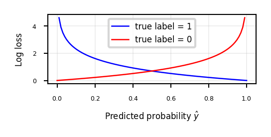
Loss function: Cross-entropy#
Models that return class probabilities can use cross-entropy loss
\[\mathcal{L_{log}}(\mathbf{w}) = \sum_{n=1}^{N} H(p_n,q_n) = - \sum_{n=1}^{N} \sum_{c=1}^{C} p_{n,c} log(q_{n,c}) \]Also known as log loss, logistic loss, or maximum likelihood
Based on true probabilities \(p\) (0 or 1) and predicted probabilities \(q\) over \(N\) instances and \(C\) classes
Binary case (C=2): \(\mathcal{L_{log}}(\mathbf{w}) = - \sum_{n=1}^{N} \big[ y_n log(\hat{y}_n) + (1-y_n) log(1-\hat{y}_n) \big]\)
Penalty (a.k.a. ‘surprise’) grows exponentially as difference between \(p\) and \(q\) increases
If you are sure of an answer (high \(q\)) and it’s wrong (low \(p\)), you definitely want to learn
Often used together with L2 (or L1) loss: \(\mathcal{L_{log}}'(\mathbf{w}) = \mathcal{L_{log}}(\mathbf{w}) + \alpha \sum_{i} w_i^2 \)
Show code cell source
def cross_entropy(yHat, y):
    if y == 1:
        return -np.log(yHat)
    else:
        return -np.log(1 - yHat)

fig, ax = plt.subplots(figsize=(6*fig_scale,2*fig_scale))
x = np.linspace(0,1,100)

ax.plot(x,cross_entropy(x, 1),lw=2*fig_scale,c='b',label='true label = 1', linestyle='-')
ax.plot(x,cross_entropy(x, 0),lw=2*fig_scale,c='r',label='true label = 0', linestyle='-')
ax.set_xlabel(r"Predicted probability $\hat{y}$")
ax.set_ylabel("Log loss")
plt.grid()
plt.legend();
Optimization methods (solvers) for cross-entropy loss#
Gradient descent (only supports L2 regularization)
Log loss is differentiable, so we can use (stochastic) gradient descent
Variants thereof, e.g. Stochastic Average Gradient (SAG, SAGA)
Coordinate descent (supports both L1 and L2 regularization)
Faster iteration, but may converge more slowly, has issues with saddlepoints
Called
liblinearin sklearn. Can’t run in parallel.
Newton-Rhapson or Newton Conjugate Gradient (only L2):
Uses the Hessian \(H = \big[\frac{\partial^2 \mathcal{L}}{\partial x_i \partial x_j} \big]\): \(\mathbf{w}^{s+1} = \mathbf{w}^s-\eta H^{-1}(\mathbf{w}^s) \nabla \mathcal{L}(\mathbf{w}^s)\)
Slow for large datasets. Works well if solution space is (near) convex
Quasi-Newton methods (only L2)
Approximate, faster to compute
E.g. Limited-memory Broyden–Fletcher–Goldfarb–Shanno (
lbfgs)Default in sklearn for Logistic Regression
Some hints on choosing solvers
Data scaling helps convergence, minimizes differences between solvers
In practice#
Logistic regression can also be found in
sklearn.linear_model.Chyperparameter is the inverse regularization strength: \(C=\alpha^{-1}\)penalty: type of regularization: L1, L2 (default), Elastic-Net, or Nonesolver: newton-cg, lbfgs (default), liblinear, sag, saga
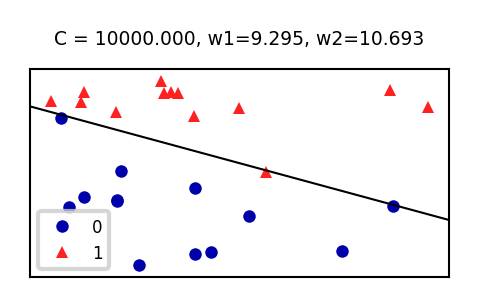
Increasing C: less regularization, tries to overfit individual points
from sklearn.linear_model import LogisticRegression
lr = LogisticRegression(C=1).fit(X_train, y_train)
Show code cell source
from sklearn.linear_model import LogisticRegression

@interact
def plot_lr(C_log=(-3,4,0.1)):
    # Still using artificial data
    fig, ax = plt.subplots(figsize=(6*fig_scale,3*fig_scale))
    mglearn.discrete_scatter(Xf[:, 0], Xf[:, 1], yf, ax=ax, s=10*fig_scale)
    lr = LogisticRegression(C=10**C_log).fit(Xf, yf)
    w = lr.coef_[0]
    xx = np.linspace(7, 13)
    yy = (-w[0] * xx - lr.intercept_[0]) / w[1]
    ax.plot(xx, yy, c='k')
    ax.set_xticks(())
    ax.set_yticks(())
    ax.set_title("C = {:.3f}, w1={:.3f}, w2={:.3f}".format(10**C_log,w[0],w[1]))
    ax.legend(loc="best");
    plt.show()
Show code cell source
if not interactive:
    plot_lr(C_log=(4))
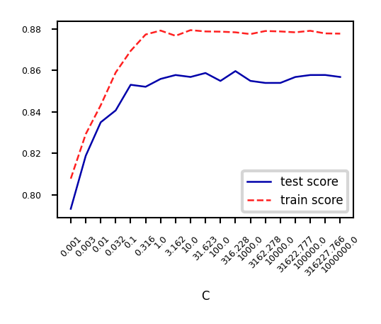
Analyze behavior on the breast cancer dataset
Underfitting if C is too small, some overfitting if C is too large
We use cross-validation because the dataset is small
Show code cell source
from sklearn.datasets import fetch_openml
from sklearn.model_selection import cross_validate

spam_data = fetch_openml(name="qsar-biodeg", as_frame=True)
X_C, y_C = spam_data.data, spam_data.target

C=np.logspace(-3,6,num=19)
test_score=[]
train_score=[]
for c in C:
    lr = LogisticRegression(C=c)
    scores = cross_validate(lr,X_C,y_C,cv=10, return_train_score=True)
    test_score.append(np.mean(scores['test_score']))
    train_score.append(np.mean(scores['train_score']))
fig, ax = plt.subplots(figsize=(6*fig_scale,4*fig_scale))
ax.set_xticks(range(19))
ax.set_xticklabels(np.round(C,3))
ax.set_xlabel('C')
ax.plot(test_score, lw=2*fig_scale, label='test score')
ax.plot(train_score, lw=2*fig_scale, label='train score')
ax.legend()
plt.xticks(rotation=45);
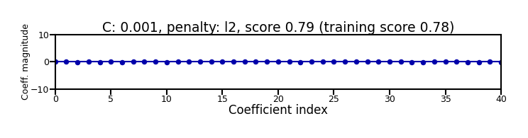
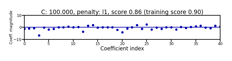
Again, choose between L1 or L2 regularization (or elastic-net)
Small C overfits, L1 leads to sparse models
Show code cell source
X_C_train, X_C_test, y_C_train, y_C_test = train_test_split(X_C, y_C, random_state=0)

@interact
def plot_logreg(C=(0.01,1000.0,0.1), penalty=['l1','l2']):
    r = LogisticRegression(C=C, penalty=penalty, solver='liblinear').fit(X_C_train, y_C_train)
    fig, ax = plt.subplots(figsize=(8*fig_scale,1.9*fig_scale))
    ax.plot(r.coef_.T, 'o', markersize=6*fig_scale)
    ax.set_title("C: {:.3f}, penalty: {}, score {:.2f} (training score {:.2f})".format(C, penalty, r.score(X_C_test, y_C_test), r.score(X_C_train, y_C_train)),pad=0)
    ax.set_xlabel("Coefficient index", labelpad=0)
    ax.set_ylabel("Coeff. magnitude", labelpad=0, fontsize=10*fig_scale)
    ax.tick_params(axis='both', pad=0)
    ax.hlines(0, 40, len(r.coef_)-1)
    ax.set_ylim(-10, 10)
    ax.set_xlim(0, 40);
    plt.tight_layout();
    plt.show();
Show code cell source
if not interactive:
    plot_logreg(0.001, 'l2')
    plot_logreg(100, 'l2')
    plot_logreg(100, 'l1')

Ridge Classification#
Instead of log loss, we can also use ridge loss:
\[\mathcal{L}_{Ridge} = \sum_{n=1}^{N} (y_n-(\mathbf{w}\mathbf{x_n} + w_0))^2 + \alpha \sum_{i=1}^{p} w_i^2\]In this case, target values {negative, positive} are converted to {-1,1}
Can be solved similarly to Ridge regression:
Closed form solution (a.k.a. Cholesky)
Gradient descent and variants
E.g. Conjugate Gradient (CG) or Stochastic Average Gradient (SAG,SAGA)
Use Cholesky for smaller datasets, Gradient descent for larger ones
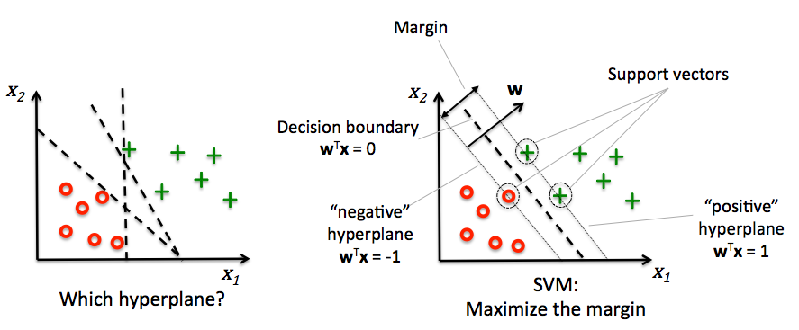
Support vector machines#
Decision boundaries close to training points may generalize badly
Very similar (nearby) test point are classified as the other class
Choose a boundary that is as far away from training points as possible
The support vectors are the training samples closest to the hyperplane
The margin is the distance between the separating hyperplane and the support vectors
Hence, our objective is to maximize the margin
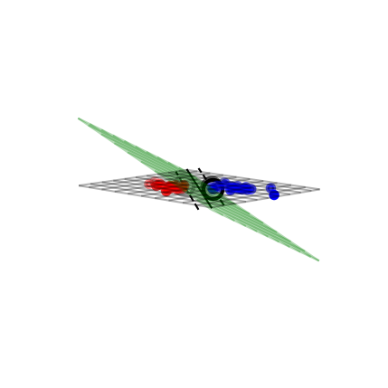
Solving SVMs with Lagrange Multipliers#
Imagine a hyperplane (green) \(y= \sum_1^p \mathbf{w}_i * \mathbf{x}_i + w_0\) that has slope \(\mathbf{w}\), value ‘+1’ for the positive (red) support vectors, and ‘-1’ for the negative (blue) ones
Margin between the boundary and support vectors is \(\frac{y-w_0}{||\mathbf{w}||}\), with \(||\mathbf{w}|| = \sum_i^p w_i^2\)
We want to find the weights that maximize \(\frac{1}{||\mathbf{w}||}\). We can also do that by maximizing \(\frac{1}{||\mathbf{w}||^2}\)
Show code cell source
from sklearn.svm import SVC

# we create 40 separable points
np.random.seed(0)
sX = np.r_[np.random.randn(20, 2) - [2, 2], np.random.randn(20, 2) + [2, 2]]
sY = [0] * 20 + [1] * 20

# fit the model
s_clf = SVC(kernel='linear')
s_clf.fit(sX, sY)

@interact
def plot_svc_fit(rotationX=(0,20,1),rotationY=(90,180,1)):
    # get the separating hyperplane
    w = s_clf.coef_[0]
    a = -w[0] / w[1]
    xx = np.linspace(-5, 5)
    yy = a * xx - (s_clf.intercept_[0]) / w[1]
    zz = np.linspace(-2, 2, 30)

    # plot the parallels to the separating hyperplane that pass through the
    # support vectors
    b = s_clf.support_vectors_[0]
    yy_down = a * xx + (b[1] - a * b[0])
    b = s_clf.support_vectors_[-1]
    yy_up = a * xx + (b[1] - a * b[0])

    # plot the line, the points, and the nearest vectors to the plane
    fig = plt.figure(figsize=(7*fig_scale,4.5*fig_scale))
    ax = plt.axes(projection="3d")
    ax.plot3D(xx, yy, [0]*len(xx), 'k-')
    ax.plot3D(xx, yy_down, [0]*len(xx), 'k--')
    ax.plot3D(xx, yy_up, [0]*len(xx), 'k--')

    ax.scatter3D(s_clf.support_vectors_[:, 0], s_clf.support_vectors_[:, 1], [0]*len(s_clf.support_vectors_[:, 0]),
                s=85*fig_scale, edgecolors='k', c='w')
    ax.scatter3D(sX[:, 0], sX[:, 1], [0]*len(sX[:, 0]), c=sY, cmap=plt.cm.bwr, s=10*fig_scale )


    # Planes
    XX, YY = np.meshgrid(xx, yy)
    if interactive:
        ZZ = w[0]*XX+w[1]*YY+clf.intercept_[0]
    else: # rescaling (for prints) messes up the Z values
        ZZ = w[0]*XX/fig_scale+w[1]*YY/fig_scale+clf.intercept_[0]*fig_scale/2
    ax.plot_wireframe(XX, YY, XX*0, rstride=5, cstride=5, alpha=0.3, color='k', label='XY plane')
    ax.plot_wireframe(XX, YY, ZZ, rstride=5, cstride=5, alpha=0.3, color='g', label='hyperplane')

    ax.set_axis_off()
    ax.view_init(rotationX, rotationY) # Use this to rotate the figure
    ax.dist = 6
    plt.tight_layout()
    plt.show()
Show code cell source
if not interactive:
    plot_svc_fit(9,135)
Geometric interpretation#
We want to maximize \(f = \frac{1}{||w||^2}\) (blue contours)
The hyperplane (red) must be \(> 1\) for all positive examples:
\(g(\mathbf{w}) = \mathbf{w} \mathbf{x_i} + w_0 > 1 \,\,\, \forall{i}, y(i)=1\)Find the weights \(\mathbf{w}\) that satify \(g\) but maximize \(f\)
Solution#
A quadratic loss function with linear constraints can be solved with Lagrangian multipliers
This works by assigning a weight \(a_i\) (called a dual coefficient) to every data point \(x_i\)
They reflect how much individual points influence the weights \(\mathbf{w}\)
The points with non-zero \(a_i\) are the support vectors
Next, solve the following Primal objective:
\(y_i=\pm1\) is the correct class for example \(x_i\)
so that
It has a Dual formulation as well (See ‘Elements of Statistical Learning’ for the full derivation):
so that
Computes the dual coefficients directly. A number \(l\) of these are non-zero (sparseness).
Dot product \(\mathbf{x_i} \mathbf{x_j}\) can be interpreted as the closeness between points \(\mathbf{x_i}\) and \(\mathbf{x_j}\)
We can replace the dot product with other similarity functions (kernels)
\(\mathcal{L}_{Dual}\) increases if nearby support vectors \(\mathbf{x_i}\) with high weights \(a_i\) have different class \(y_i\)
\(\mathcal{L}_{Dual}\) also increases with the number of support vectors \(l\) and their weights \(a_i\)
Can be solved with quadratic programming, e.g. Sequential Minimal Optimization (SMO)
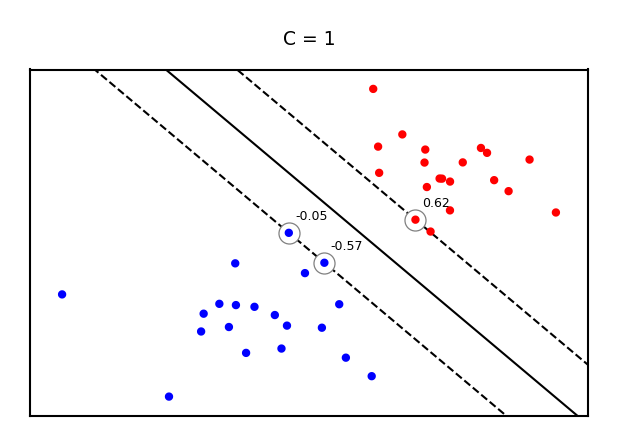
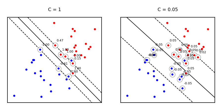
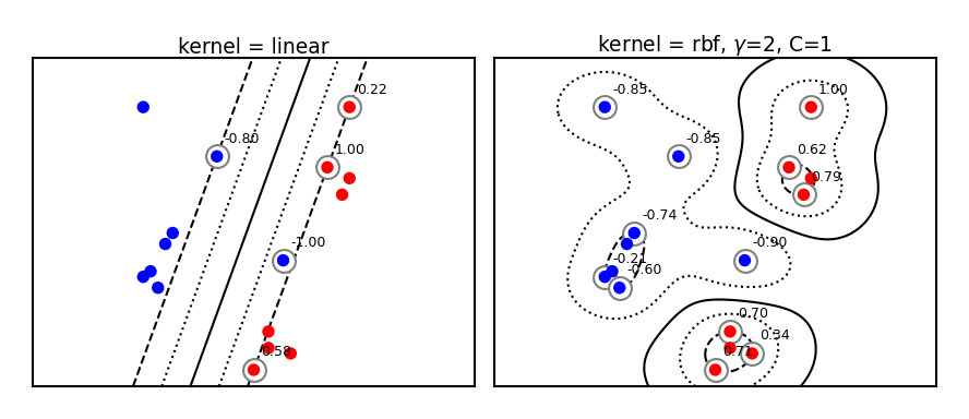
Example result. The circled samples are support vectors, together with their coefficients.
Show code cell source
from sklearn.svm import SVC

# Plot SVM support vectors
def plot_linear_svm(X,y,C,ax):

    clf = SVC(kernel='linear', C=C)
    clf.fit(X, y)

    # get the separating hyperplane
    w = clf.coef_[0]
    a = -w[0] / w[1]
    xx = np.linspace(-5, 5)
    yy = a * xx - (clf.intercept_[0]) / w[1]

    # plot the parallels to the separating hyperplane
    yy_down = (-1-w[0]*xx-clf.intercept_[0])/w[1]
    yy_up = (1-w[0]*xx-clf.intercept_[0])/w[1]

    # plot the line, the points, and the nearest vectors to the plane
    ax.set_title('C = %s' % C)
    ax.plot(xx, yy, 'k-')
    ax.plot(xx, yy_down, 'k--')
    ax.plot(xx, yy_up, 'k--')
    ax.scatter(clf.support_vectors_[:, 0], clf.support_vectors_[:, 1],
                s=85*fig_scale, edgecolors='gray', c='w', zorder=10, lw=1*fig_scale)
    ax.scatter(X[:, 0], X[:, 1], c=y, zorder=10, cmap=plt.cm.bwr)
    ax.axis('tight')

    # Add coefficients
    for i, coef in enumerate(clf.dual_coef_[0]):
        ax.annotate("%0.2f" % (coef), (clf.support_vectors_[i, 0]+0.1,clf.support_vectors_[i, 1]+0.35), fontsize=10*fig_scale, zorder=11)

    ax.set_xlim(np.min(X[:, 0])-0.5, np.max(X[:, 0])+0.5)
    ax.set_ylim(np.min(X[:, 1])-0.5, np.max(X[:, 1])+0.5)
    ax.set_xticks(())
    ax.set_yticks(())


# we create 40 separable points
np.random.seed(0)
svm_X = np.r_[np.random.randn(20, 2) - [2, 2], np.random.randn(20, 2) + [2, 2]]
svm_Y = [0] * 20 + [1] * 20
svm_fig, svm_ax = plt.subplots(figsize=(8*fig_scale,5*fig_scale))
plot_linear_svm(svm_X,svm_Y,1,svm_ax)
Making predictions#
\(a_i\) will be 0 if the training point lies on the right side of the decision boundary and outside the margin
The training samples for which \(a_i\) is not 0 are the support vectors
Hence, the SVM model is completely defined by the support vectors and their dual coefficients (weights)
Knowing the dual coefficients \(a_i\), we can find the weights \(w\) for the maximal margin separating hyperplane
And we could classify a new sample \(\mathbf{u}\) by looking at the sign of \(\mathbf{w}\mathbf{u}+w_0\)
However, we don’t need to compute \(\mathbf{w}\) to make predictions. We only need to look at the support vectors.
SVMs and kNN#
Remember, we will classify a new point \(\mathbf{u}\) by looking at the sign of:
Weighted k-nearest neighbor is a generalization of the k-nearest neighbor classifier. It classifies points by evaluating:
Hence: SVM’s predict much the same way as k-NN, only:
They only consider the truly important points (the support vectors): much faster
The number of neighbors is the number of support vectors
The distance function is an inner product of the inputs (or another kernel)
Given \(\mathbf{u}\), we predict by looking at the classes of the support vectors, weighted by their distance.
Regularized (soft margin) SVMs#
If the data is not linearly separable, (hard) margin maximization becomes meaningless
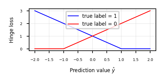
Relax the contraint by allowing an error \(\xi_{i}\): \(y_i (\mathbf{w}\mathbf{x_i} + w_0) \geq 1 - \xi_{i}\)
Or (since \(\xi_{i} \geq 0\)): \(\xi_{i} = max(0,1-y_i\cdot(\mathbf{w}\mathbf{x_i} + w_0))\)
The sum over all points is called hinge loss: \(\sum_i^n \xi_{i}\)
Attenuating the error component with a hyperparameter \(C\), we get the objective
Can still be solved with quadratic programming
Show code cell source
def hinge_loss(yHat, y):
    if y == 1:
        return np.maximum(0,1-yHat)
    else:
        return np.maximum(0,1+yHat)

fig, ax = plt.subplots(figsize=(6*fig_scale,2*fig_scale))
x = np.linspace(-2,2,100)

ax.plot(x,hinge_loss(x, 1),lw=2*fig_scale,c='b',label='true label = 1', linestyle='-')
ax.plot(x,hinge_loss(x, 0),lw=2*fig_scale,c='r',label='true label = 0', linestyle='-')
ax.set_xlabel(r"Prediction value $\hat{y}$")
ax.set_ylabel("Hinge loss")
plt.grid()
plt.legend();
Sidenote: Least Squares SVMs#
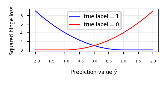
We can also use the squares of all the errors, or squared hinge loss: \(\sum_i^n \xi_{i}^2\)
This yields the Least Squares SVM objective
Can be solved with Lagrangian Multipliers and a set of linear equations
Still yields support vectors and still allows kernelization
Support vectors are not sparse, but pruning techniques exist
Show code cell source
fig, ax = plt.subplots(figsize=(6*fig_scale,2*fig_scale))
x = np.linspace(-2,2,100)

ax.plot(x,hinge_loss(x, 1)** 2,lw=2*fig_scale,c='b',label='true label = 1', linestyle='-')
ax.plot(x,hinge_loss(x, 0)** 2,lw=2*fig_scale,c='r',label='true label = 0', linestyle='-')
ax.set_xlabel(r"Prediction value $\hat{y}$")
ax.set_ylabel("Squared hinge loss")
plt.grid()
plt.legend();
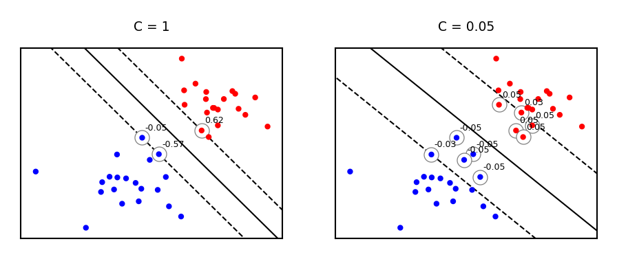
Effect of regularization on margin and support vectors#
SVM’s Hinge loss acts like L1 regularization, yields sparse models
C is the inverse regularization strength (inverse of \(\alpha\) in Lasso)
Larger C: fewer support vectors, smaller margin, more overfitting
Smaller C: more support vectors, wider margin, less overfitting
Needs to be tuned carefully to the data
Show code cell source
fig, svm_axes = plt.subplots(nrows=1, ncols=2, figsize=(12*fig_scale, 4*fig_scale))
plot_linear_svm(svm_X,svm_Y,1,svm_axes[0])
plot_linear_svm(svm_X,svm_Y,0.05,svm_axes[1])
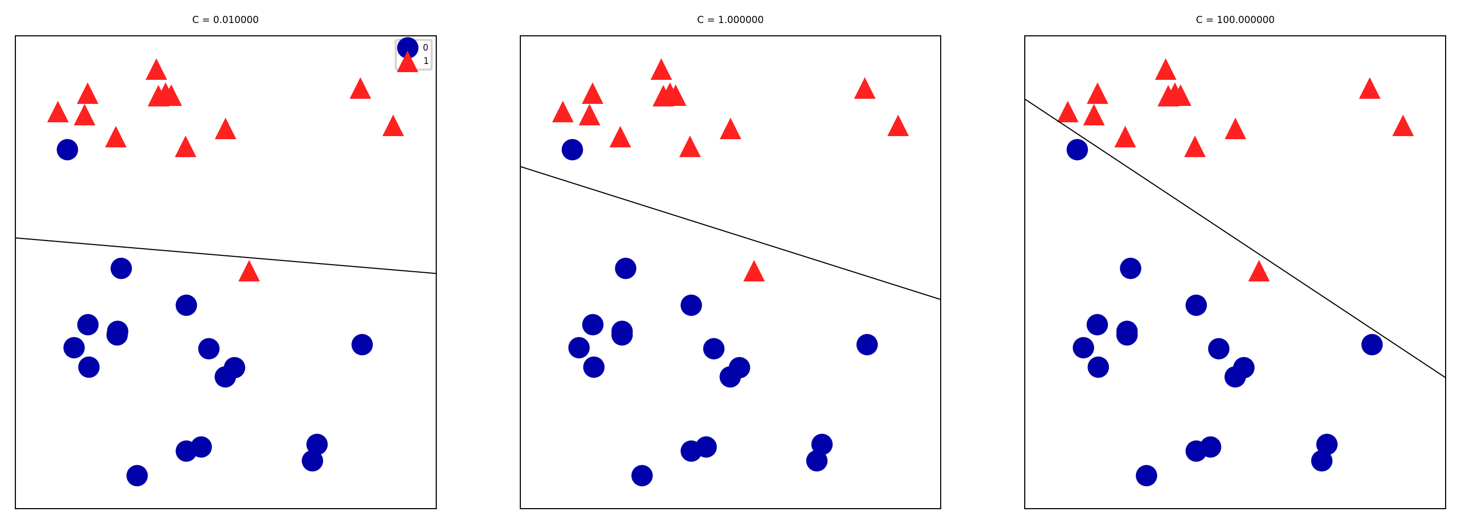
Same for non-linearly separable data
Show code cell source
svm_X = np.r_[np.random.randn(20, 2) - [1, 1], np.random.randn(20, 2) + [1, 1]]
fig, svm_axes = plt.subplots(nrows=1, ncols=2, figsize=(12*fig_scale, 5*fig_scale))
plot_linear_svm(svm_X,svm_Y,1,svm_axes[0])
plot_linear_svm(svm_X,svm_Y,0.05,svm_axes[1])
Large C values can lead to overfitting (e.g. fitting noise), small values can lead to underfitting
Show code cell source
mglearn.plots.plot_linear_svc_regularization()
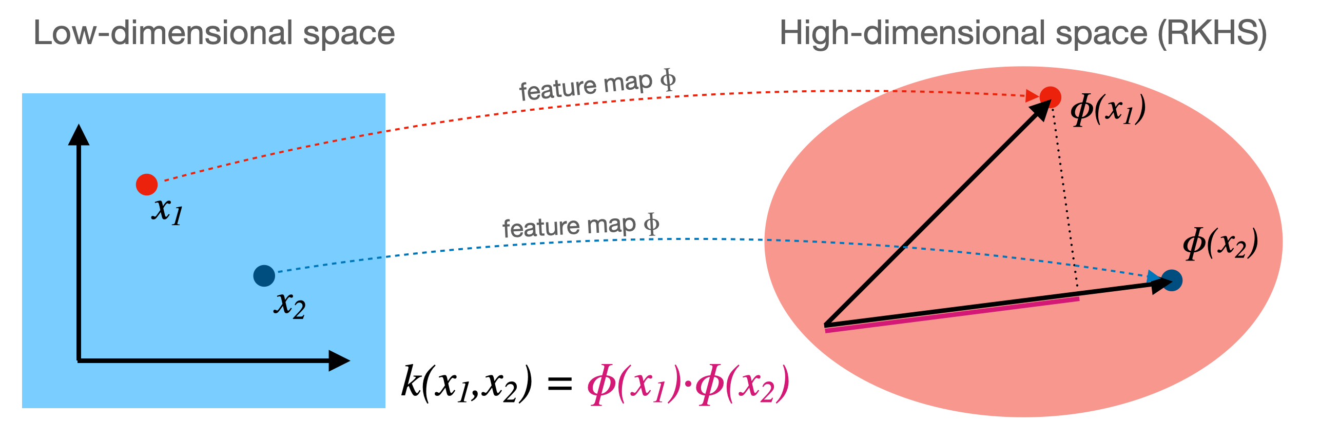
Kernelization#
Sometimes we can separate the data better by first transforming it to a higher dimensional space \(\Phi(x)\)
This transformation \(\Phi\) is called a feature map (but can be expensive)
For certain \(\Phi\), we know the function \(k\) that computes the dot product in \(\Phi(x)\): \( k(\mathbf{x_i},\mathbf{x_j}) = \Phi(\mathbf{x_i}) \cdot \Phi(\mathbf{x_j})\)
This kernel function \(k(\mathbf{x_i},\mathbf{x_j})\) computes the dot product without having to construct (reproduce) \(\Phi(x)\)
Kernel trick: if your loss function has a dot product, you can simply replace it with a kernel!
For SVMs (in dual form), replacing \((\mathbf{x_i}\mathbf{x_j}) \rightarrow k(\mathbf{x_i},\mathbf{x_j})\) yields a kernelized SVM: $\(\mathcal{L}_{Dual} (a_i, k) = \sum_{i=1}^{l} a_i - \frac{1}{2} \sum_{i,j=1}^{l} a_i a_j y_i y_j k(\mathbf{x_i},\mathbf{x_j}) \)$
Polynomial kernel#
The polynomial kernel (for degree \(d \in \mathbb{N}\)) reproduces the polynomial feature map
It can be easily computed from the original dot product:
It has two more hyperparameters, but you can usually leave them at default
\(\gamma\) is a scaling hyperparameter (default \(\frac{1}{p}\))
\(c_0\) is a hyperparameter (default 1) to trade off influence of higher-order terms
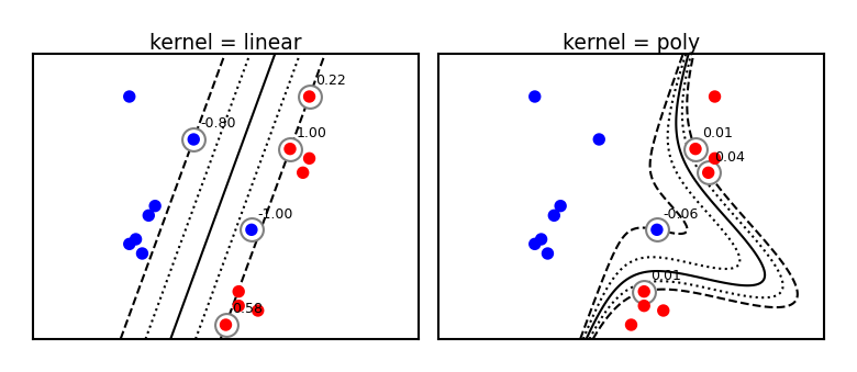
By simply replacing the dot product with a kernel we can learn non-linear SVMs!
It is technically still linear in \(\Phi(x)\), but in our original space the boundary becomes a polynomial curve
Prediction still happens as before, but the influence of each support vector drops of polynomially (with degree \(d\))
from sklearn import svm

def plot_svm_kernels(kernels, poly_degree=3, gamma=2, C=1, size=4):
    # Our dataset and targets
    X = np.c_[(.4, -.7),
              (-1.5, -1),
              (-1.4, -.9),
              (-1.3, -1.2),
              (-1.1, -.2),
              (-1.2, -.4),
              (-.5, 1.2),
              (-1.5, 2.1),
              (1, 1),
              # --
              (1.3, .8),
              (1.2, .5),
              (.2, -2),
              (.5, -2.4),
              (.2, -2.3),
              (0, -2.7),
              (1.3, 2.1)].T
    Y = [0] * 8 + [1] * 8

    # figure number
    fig, axes = plt.subplots(-(-len(kernels)//3), min(len(kernels),3), figsize=(min(len(kernels),3)*size*1.2*fig_scale, -(-len(kernels)//3)*size*fig_scale), tight_layout=True)
    if len(kernels) == 1:
        axes = np.array([axes])
    if not isinstance(gamma,list):
        gamma = [gamma]*len(kernels)
    if not isinstance(C,list):
        C = [C]*len(kernels)
    # fit the model
    for kernel, ax, g, c in zip(kernels,axes.reshape(-1),gamma,C):
        clf = svm.SVC(kernel=kernel, gamma=g, C=c, degree=poly_degree)
        clf.fit(X, Y)

        # plot the line, the points, and the nearest vectors to the plane
        if kernel == 'rbf':
            ax.set_title(r"kernel = {}, $\gamma$={}, C={}".format(kernel, g, c), pad=0.1)
        else:
            ax.set_title('kernel = %s' % kernel,pad=0.1)

        ax.scatter(clf.support_vectors_[:, 0], clf.support_vectors_[:, 1],
                    s=25, edgecolors='grey', c='w', zorder=10, linewidths=0.5)
        ax.scatter(X[:, 0], X[:, 1], c=Y, zorder=10, cmap=plt.cm.bwr, s=10*fig_scale)

        for i, coef in enumerate(clf.dual_coef_[0]):
            ax.annotate("%0.2f" % (coef), (clf.support_vectors_[i, 0]+0.1,clf.support_vectors_[i, 1]+0.25), zorder=11, fontsize=3)

        ax.axis('tight')
        x_min = -3
        x_max = 3
        y_min = -3
        y_max = 3

        XX, YY = np.mgrid[x_min:x_max:200j, y_min:y_max:200j]
        Z = clf.decision_function(np.c_[XX.ravel(), YY.ravel()])

        # Put the result into a color plot
        Z = Z.reshape(XX.shape)
        #plt.pcolormesh(XX, YY, Z > 0, cmap=plt.cm.bwr, alpha=0.1)
        ax.contour(XX, YY, Z, colors=['k', 'k', 'k', 'k', 'k'], linestyles=['--', ':', '-', ':', '--'],
                    levels=[-1, -0.5, 0, 0.5, 1])

        ax.set_xlim(x_min, x_max)
        ax.set_ylim(y_min, y_max)

        ax.set_xticks([])
        ax.set_yticks([])

    plt.tight_layout()
    plt.show()
plot_svm_kernels(['linear', 'poly'],poly_degree=3,size=3.5)
Radial Basis Function (RBF) kernel#
The RBF or Gaussian kernel (of width \(\gamma > 0\)) is related to the Taylor series expansion of \(e^x\)
It is a function of how closely together two data points are:
The influence of a point \(\mathbf{x_2}\) on point \(\mathbf{x_1}\) drops off exponentially with its distance to \(\mathbf{x_1}\)
The influence of each support vector now drops of exponentially
Hence, predictions are only affected by very nearby support vectors
RBF kernels are therefore called local kernels
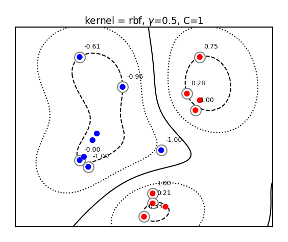
plot_svm_kernels(['linear', 'rbf'],poly_degree=3,gamma=2,size=4)
The kernel width (\(\gamma\)) defines how sharply the local influence decays
Acts as a regularizer: low \(\gamma\) causes underfitting and high \(\gamma\) causes overfitting
SVM’s C parameter (inverse regularizer) is still at play and thus interacts with \(\gamma\)
@interact
def plot_rbf_data(gamma=(0.1,10,0.5),C=(0.01,5,0.1)):
    plot_svm_kernels(['rbf'],gamma=gamma,C=C,size=5)
if not interactive:
    plot_svm_kernels(['rbf'],gamma=0.5,C=1,size=5)
Kernelization sidenotes (optional)#
You can invent many more feature maps and corresponding kernels (eg. for text, graphs,…)
However, learning deep learning embeddings from lots of data often works better
You can also kernelize Ridge regression, Logistic regression, Perceptrons, Support Vector Regression,…
The Representer theorem will give you the corresponding loss function
For more detail see the Kernelization lecture under extra materials.
SVMs in scikit-learn#
svm.LinearSVC: faster for large datasetsAllows choosing between the primal or dual. Primal recommended when \(n\) >> \(p\)
Returns
coef_(\(\mathbf{w}\)) andintercept_(\(w_0\))
svm.SVCallows different kernels to be usedAlso returns
support_vectors_(the support vectors) and thedual_coef_\(a_i\)Scales at least quadratically with the number of samples \(n\)
svm.LinearSVRandsvm.SVRare variants for regression
clf = svm.SVC(kernel='linear') # or 'RBF' or 'Poly'
clf.fit(X, Y)
print("Support vectors:", clf.support_vectors_[:])
print("Coefficients:", clf.dual_coef_[:])
Show code cell source
from sklearn import svm

# Linearly separable dat
np.random.seed(0)
X = np.r_[np.random.randn(20, 2) - [2, 2], np.random.randn(20, 2) + [2, 2]]
Y = [0] * 20 + [1] * 20

# Fit the model
clf = svm.SVC(kernel='linear')
clf.fit(X, Y)

# Get the support vectors and weights
print("Support vectors:")
print(clf.support_vectors_[:])
print("Coefficients:")
print(clf.dual_coef_[:])
Support vectors:
[[-1.021  0.241]
 [-0.467 -0.531]
 [ 0.951  0.58 ]]
Coefficients:
[[-0.048 -0.569  0.617]]
Solving SVMs with Gradient Descent#
SVMs can, alternatively, be solved using gradient decent
Good for large datasets, but does not yield support vectors or kernelization
Hinge loss is not differentiable but convex, and has a subgradient:
Can be solved with (stochastic) gradient descent
Generalized SVMs#
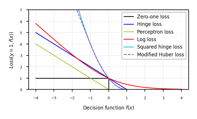
There are many smoothed versions of hinge loss:
Squared hinge loss:
Also known as Ridge classification
Least Squares SVM: allows kernelization (using a linear equation solver)
Modified Huber loss: squared hinge, but linear after -1. Robust against outliers
Log loss: equivalent to logistic regression
In sklearn,
SGDClassifiercan be used with any of these. Good for large datasets.
Show code cell source
def modified_huber_loss(y_true, y_pred):
    z = y_pred * y_true
    loss = -4 * z
    loss[z >= -1] = (1 - z[z >= -1]) ** 2
    loss[z >= 1.] = 0
    return loss

xmin, xmax = -4, 4
xx = np.linspace(xmin, xmax, 100)
lw = 2*fig_scale
fig, ax = plt.subplots(figsize=(8*fig_scale,4*fig_scale))
plt.plot([xmin, 0, 0, xmax], [1, 1, 0, 0], 'k-', lw=lw,
         label="Zero-one loss")
plt.plot(xx, np.where(xx < 1, 1 - xx, 0), 'b-', lw=lw,
         label="Hinge loss")
plt.plot(xx, -np.minimum(xx, 0), color='yellowgreen', lw=lw,
         label="Perceptron loss")
plt.plot(xx, np.log2(1 + np.exp(-xx)), 'r-', lw=lw,
         label="Log loss")
plt.plot(xx, np.where(xx < 1, 1 - xx, 0) ** 2, 'c-', lw=lw,
         label="Squared hinge loss")
plt.plot(xx, modified_huber_loss(xx, 1), color='darkorchid', lw=lw,
         linestyle='--', label="Modified Huber loss")
plt.ylim((0, 7))
plt.legend(loc="upper right")
plt.xlabel(r"Decision function $f(x)$")
plt.ylabel("$Loss(y=1, f(x))$")
plt.grid()
plt.legend();
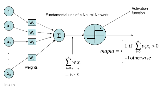
Perceptron#
Represents a single neuron (node) with inputs \(x_i\), a bias \(w_0\), and output \(y\)
Each connection has a (synaptic) weight \(w_i\). The node outputs \(\hat{y} = \sum_{i}^n x_{i}w_i + w_0\)
The activation function (neuron output) is 1 if \(\mathbf{xw} + w_0 > 0\), -1 otherwise
Idea: Update synapses only on misclassification, correct output by exactly \(\pm1\)
Weights can be learned with (stochastic) gradient descent and Hinge(0) loss
\[\mathcal{L}_{Perceptron} = max(0,-y_i (\mathbf{w}\mathbf{x_i} + w_0))\]\[\begin{split}\frac{\partial \mathcal{L_{Perceptron}}}{\partial w_i} = \begin{cases}-y_i x_i & y_i (\mathbf{w}\mathbf{x_i} + w_0) < 0\\ 0 & \text{otherwise} \\ \end{cases}\end{split}\]
Linear Models for multiclass classification#
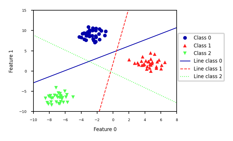
one-vs-rest (aka one-vs-all)#
Learn a binary model for each class vs. all other classes
Create as many binary models as there are classes
Show code cell source
from sklearn.datasets import make_blobs

X, y = make_blobs(random_state=42)
linear_svm = LinearSVC().fit(X, y)

plt.rcParams["figure.figsize"] = (7*fig_scale,5*fig_scale)
mglearn.discrete_scatter(X[:, 0], X[:, 1], y, s=10*fig_scale)
line = np.linspace(-15, 15)
for coef, intercept, color in zip(linear_svm.coef_, linear_svm.intercept_,
                                  mglearn.cm3.colors):
    plt.plot(line, -(line * coef[0] + intercept) / coef[1], c=color, lw=2*fig_scale)
plt.ylim(-10, 15)
plt.xlim(-10, 8)
plt.xlabel("Feature 0")
plt.ylabel("Feature 1")
plt.legend(['Class 0', 'Class 1', 'Class 2', 'Line class 0', 'Line class 1',
            'Line class 2'], loc=(1.01, 0.3));
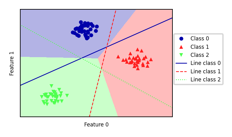
Every binary classifiers makes a prediction, the one with the highest score (>0) wins
Show code cell source
mglearn.plots.plot_2d_classification(linear_svm, X, fill=True, alpha=0.3)
mglearn.discrete_scatter(X[:, 0], X[:, 1], y, s=10*fig_scale)
line = np.linspace(-15, 15)
for coef, intercept, color in zip(linear_svm.coef_, linear_svm.intercept_,
                                  mglearn.cm3.colors):
    plt.plot(line, -(line * coef[0] + intercept) / coef[1], c=color, lw=2*fig_scale)
plt.legend(['Class 0', 'Class 1', 'Class 2', 'Line class 0', 'Line class 1',
            'Line class 2'], loc=(1.01, 0.3))
plt.xlabel("Feature 0")
plt.ylabel("Feature 1");
one-vs-one#
An alternative is to learn a binary model for every combination of two classes
For \(C\) classes, this results in \(\frac{C(C-1)}{2}\) binary models
Each point is classified according to a majority vote amongst all models
Can also be a ‘soft vote’: sum up the probabilities (or decision values) for all models. The class with the highest sum wins.
Requires more models than one-vs-rest, but training each one is faster
Only the examples of 2 classes are included in the training data
Recommended for algorithms than learn well on small datasets
Especially SVMs and Gaussian Processes
Show code cell source
%%HTML
<style>
td {font-size: 16px}
th {font-size: 16px}
.rendered_html table, .rendered_html td, .rendered_html th {
    font-size: 16px;
}
</style>
Linear models overview#
Name |
Representation |
Loss function |
Optimization |
Regularization |
|---|---|---|---|---|
Least squares |
Linear function (R) |
SSE |
CFS or SGD |
None |
Ridge |
Linear function (R) |
SSE + L2 |
CFS or SGD |
L2 strength (\(\alpha\)) |
Lasso |
Linear function (R) |
SSE + L1 |
Coordinate descent |
L1 strength (\(\alpha\)) |
Elastic-Net |
Linear function (R) |
SSE + L1 + L2 |
Coordinate descent |
\(\alpha\), L1 ratio (\(\rho\)) |
SGDRegressor |
Linear function (R) |
SSE, Huber, \(\epsilon\)-ins,… + L1/L2 |
SGD |
L1/L2, \(\alpha\) |
Logistic regression |
Linear function (C) |
Log + L1/L2 |
SGD, coordinate descent,… |
L1/L2, \(\alpha\) |
Ridge classification |
Linear function (C) |
SSE + L2 |
CFS or SGD |
L2 strength (\(\alpha\)) |
Linear SVM |
Support Vectors |
Hinge(1) |
Quadratic programming or SGD |
Cost (C) |
Kernelized SVM |
Support Vectors |
Hinge(1) |
Quadratic programming or SGD |
Cost (C), \(\gamma\),… |
Least Squares SVM |
Support Vectors |
Squared Hinge |
Linear equations or SGD |
Cost (C) |
Perceptron |
Linear function (C) |
Hinge(0) |
SGD |
None |
SGDClassifier |
Linear function (C) |
Log, (Sq.) Hinge, Mod. Huber,… |
SGD |
L1/L2, \(\alpha\) |
SSE: Sum of Squared Errors
CFS: Closed-form solution
SGD: (Stochastic) Gradient Descent and variants
(R)egression, (C)lassification
Summary#
Linear models
Good for very large datasets (scalable)
Good for very high-dimensional data (not for low-dimensional data)
Can be used to fit non-linear or low-dim patterns as well (see later)
Preprocessing: e.g. Polynomial or Poisson transformations
Generalized linear models (kernelization)
Regularization is important. Tune the regularization strength (\(\alpha\))
Ridge (L2): Good fit, sometimes sensitive to outliers
Lasso (L1): Sparse models: fewer features, more interpretable, faster
Elastic-Net: Trade-off between both, e.g. for correlated features
Most can be solved by different optimizers (solvers)
Closed form solutions or quadratic/linear solvers for smaller datasets
Gradient descent variants (SGD,CD,SAG,CG,…) for larger ones
Multi-class classification can be done using a one-vs-all approach