Python for scientific computing

Python has extensive packages to help with data analysis:

• numpy: matrices, linear algebra, Fourier transform, pseudorandom number generators

• scipy: advanced linear algebra and maths, signal processing, statistics

• pandas: DataFrames, data wrangling and analysis

• matplotlib: visualizations such as line charts, histograms, scatter plots.

# General imports
%matplotlib inline
import numpy as np
import pandas as pd
import matplotlib.pyplot as plt

NumPy

NumPy is the fundamental package required for high performance scientific computing in Python. It provides:

• ndarray: fast and space-efficient n-dimensional numeric array with vectorized arithmetic operations

• Functions for fast operations on arrays without having to write loops

• Linear algebra, random number generation, Fourier transform

• Integrating code written in C, C++, and Fortran (for faster operations)

pandas provides a richer, simpler interface to many operations. We’ll focus on using ndarrays here because they are heavily used in scikit-learn.

ndarrays

There are several ways to create numpy arrays.

# Convert normal Python array to 1-dimensional numpy array
np.array((1, 2, 53))

array([ 1,  2, 53])

# Convert sequences of sequences of sequences ... to n-dim array
np.array([(1.5, 2, 3), (4, 5, 6)])

array([[1.5, 2. , 3. ],
       [4. , 5. , 6. ]])

# Define element type at creation time
np.array([[1, 2], [3, 4]], dtype=complex)

array([[1.+0.j, 2.+0.j],
       [3.+0.j, 4.+0.j]])

Useful properties of ndarrays:

my_array = np.array([[1, 0, 3], [0, 1, 2]])
my_array.ndim     # number of dimensions (axes), also called the rank
my_array.shape    # a matrix with n rows and m columns has shape (n,m)
my_array.size     # the total number of elements of the array
my_array.dtype    # type of the elements in the array
my_array.itemsize # the size in bytes of each element of the array

8

Quick array creation.
It is cheaper to create an array with placeholders than extending it later.

np.ones(3) # Default type is float64
np.zeros([2, 2]) 
np.empty([2, 2]) # Fills the array with whatever sits in memory
np.random.random((2,3))
np.random.randint(5, size=(2, 4))

array([[4, 3, 2, 3],
       [0, 3, 4, 4]])

Create sequences of numbers

np.linspace(0, 1, num=6)   # Linearly distributed numbers between 0 and 1
np.arange(0, 1, step=0.3)  # Fixed step size
np.arange(12).reshape(3,4) # Create and reshape
np.eye(4)                  # Identity matrix

array([[1., 0., 0., 0.],
       [0., 1., 0., 0.],
       [0., 0., 1., 0.],
       [0., 0., 0., 1.]])

Basic Operations

Arithmetic operators on arrays apply elementwise. A new array is created and filled with the result. Some operations, such as += and *=, act in place to modify an existing array rather than create a new one.

a = np.array([20, 30, 40, 50])
b = np.arange(4)
a, b    # Just printing
a-b
b**2
a > 32
a += 1
a

array([21, 31, 41, 51])

The product operator * operates elementwise.
The matrix product can be performed using dot()

A, B = np.array([[1,1], [0,1]]), np.array([[2,0], [3,4]]) # assign multiple variables in one line
A
B
A * B
np.dot(A, B)

array([[5, 4],
       [3, 4]])

Upcasting: Operations with arrays of different types choose the more general/precise one.

a = np.ones(3, dtype=int) # initialize to integers
b = np.linspace(0, np.pi, 3) # default type is float
a.dtype, b.dtype, (a + b).dtype

(dtype('int64'), dtype('float64'), dtype('float64'))

ndarrays have most unary operations (max,min,sum,…) built in

a = np.random.random((2,3))
a
a.sum(), a.min(), a.max()

(0.9572624389610684, 0.06832338227931944, 0.2641917094515025)

By specifying the axis parameter you can apply an operation along a specified axis of an array

b = np.arange(12).reshape(3,4)
b
b.sum()
b.sum(axis=0) 
b.sum(axis=1) 

array([ 6, 22, 38])

Universal Functions

NumPy provides familiar mathematical functions such as sin, cos, exp, sqrt, floor,… In NumPy, these are called “universal functions” (ufunc), and operate elementwise on an array, producing an array as output.

np.sin(np.arange(0, 10))

array([ 0.        ,  0.84147098,  0.90929743,  0.14112001, -0.7568025 ,
       -0.95892427, -0.2794155 ,  0.6569866 ,  0.98935825,  0.41211849])

Shape Manipulation

Transpose, flatten, reshape,…

a = np.floor(10*np.random.random((3,4)))
a
a.transpose()
b = a.ravel() # flatten array
b
b.reshape(3, -1) # reshape in 3 rows (and as many columns as needed)

array([[0., 4., 2., 4.],
       [4., 5., 4., 6.],
       [1., 5., 3., 9.]])

Arrays can be split and stacked together

a = np.floor(10*np.random.random((2,6)))
a
b, c = np.hsplit(a, 2) # Idem: vsplit for vertical splits 
b
c
np.hstack((b, c)) # Idenm: vstack for vertical stacks

array([[0., 0., 5., 1., 7., 6.],
       [0., 2., 2., 2., 2., 8.]])

Indexing and Slicing

Arrays can be indexed and sliced using [start:stop:stepsize]. Defaults are [0:ndim:1]

a = np.arange(10)**2
a

array([ 0,  1,  4,  9, 16, 25, 36, 49, 64, 81])

a[2]

4

a[3:10:2]

array([ 9, 25, 49, 81])

a[::-1] # Defaults are used if indices not stated

array([81, 64, 49, 36, 25, 16,  9,  4,  1,  0])

a[::2]

array([ 0,  4, 16, 36, 64])

For multi-dimensional arrays, axes are comma-separated: [x,y,z].

b = np.arange(16).reshape(4,4)
b
b[2,3] # row 2, column 3

11

b[0:3,1] # Values 0 to 3 in column 1 
b[ : ,1] # The whole column 1 

array([ 1,  5,  9, 13])

b[1:3, : ] # Rows 1:3, all columns

array([[ 4,  5,  6,  7],
       [ 8,  9, 10, 11]])

# Return the last row
b[-1]   

array([12, 13, 14, 15])

Note: dots (…) represent as many colons (:) as needed

• x[1,2,…] = x[1,2,:,:,:]

• x[…,3] = x[:,:,:,:,3]

• x[4,…,5,:] = x[4,:,:,5,:]

Arrays can also be indexed by arrays of integers and booleans.

a = np.arange(12)**2         
i = np.array([ 1,1,3,8,5 ])
a
a[i]

array([ 1,  1,  9, 64, 25])

A matrix of indices returns a matrix with the corresponding values.

j = np.array([[ 3, 4], [9, 7]])
a[j]

array([[ 9, 16],
       [81, 49]])

With boolean indices we explicitly choose which items in the array we want and which ones we don’t.

a = np.arange(12).reshape(3,4)
a
a[np.array([False,True,True]), :]
b = a > 4
b
a[b]

array([ 5,  6,  7,  8,  9, 10, 11])

Iterating

Iterating is done with respect to the first axis:

for row in b:
    print(row)

[False False False False]
[False  True  True  True]
[ True  True  True  True]

Operations on each element can be done by flattening the array (or nested loops)

for element in b.flat: # flat returns an iterator 
    print(element) 

False
False
False
False
False
True
True
True
True
True
True
True

Copies and Views (or: how to shoot yourself in a foot)

Assigning an array to another variable does NOT create a copy

a = np.arange(12)
b = a
a

array([ 0,  1,  2,  3,  4,  5,  6,  7,  8,  9, 10, 11])

b[0] = -100
b

array([-100,    1,    2,    3,    4,    5,    6,    7,    8,    9,   10,
         11])

a

array([-100,    1,    2,    3,    4,    5,    6,    7,    8,    9,   10,
         11])

The view() method creates a NEW array object that looks at the same data.

a = np.arange(12)
a
c = a.view()
c.resize((2, 6))
c

array([[ 0,  1,  2,  3,  4,  5],
       [ 6,  7,  8,  9, 10, 11]])

a[0] = 123
c # c is also changed now

array([[123,   1,   2,   3,   4,   5],
       [  6,   7,   8,   9,  10,  11]])

Slicing an array returns a view of it.

c
s = c[ : , 1:3]  
s[:] = 10
s
c 

array([[123,  10,  10,   3,   4,   5],
       [  6,  10,  10,   9,  10,  11]])

The copy() method makes a deep copy of the array and its data.

d = a.copy()      
d[0] = -42
d

array([-42,  10,  10,   3,   4,   5,   6,  10,  10,   9,  10,  11])

a

array([123,  10,  10,   3,   4,   5,   6,  10,  10,   9,  10,  11])

Numpy: further reading

• Numpy Tutorial: http://wiki.scipy.org/Tentative_NumPy_Tutorial

• “Python for Data Analysis” by Wes McKinney (O’Reilly)

SciPy

SciPy is a collection of packages for scientific computing, among others:

• scipy.integrate: numerical integration and differential equation solvers

• scipy.linalg: linear algebra routines and matrix decompositions

• scipy.optimize: function optimizers (minimizers) and root finding algorithms

• scipy.signal: signal processing tools

• scipy.sparse: sparse matrices and sparse linear system solvers

• scipy.stats: probability distributions, statistical tests, descriptive statistics

Sparse matrices

Sparse matrices are used in scikit-learn for (large) arrays that contain mostly zeros. You can convert a dense (numpy) matrix to a sparse matrix.

from scipy import sparse
eye = np.eye(4)
eye
sparse_matrix = sparse.csr_matrix(eye) # Compressed Sparse Row matrix
sparse_matrix
print("{}".format(sparse_matrix))  

  (0, 0)	1.0
  (1, 1)	1.0
  (2, 2)	1.0
  (3, 3)	1.0

When the data is too large, you can create a sparse matrix by passing the values and coordinates (COO format).

data = np.ones(4)                         # [1,1,1,1]
row_indices = col_indices = np.arange(4)  # [0,1,2,3]
col_indices = np.arange(4) * 2
eye_coo = sparse.coo_matrix((data, (row_indices, col_indices)))
print("{}".format(eye_coo))

  (0, 0)	1.0
  (1, 2)	1.0
  (2, 4)	1.0
  (3, 6)	1.0

Further reading

Check the SciPy reference guide for tutorials and examples of all SciPy capabilities.

pandas

pandas is a Python library for data wrangling and analysis. It provides:

• DataFrame: a table, similar to an R DataFrame that holds any structured data

  • Every column can have its own data type (strings, dates, floats,…)

• A great range of methods to apply to this table (sorting, querying, joining,…)

• Imports data from a wide range of data formats (CSV, Excel) and databases (e.g. SQL)

Series

A one-dimensional array of data (of any numpy type), with indexed values. It can be created by passing a Python list or dict, a numpy array, a csv file,…

import pandas as pd
pd.Series([1,3,np.nan]) # Default integers are integers
pd.Series([1,3,5], index=['a','b','c'])
pd.Series({'a' : 1, 'b': 2, 'c': 3 }) # when given a dict, the keys will be used for the index
pd.Series({'a' : 1, 'b': 2, 'c': 3 }, index = ['b', 'c', 'd']) # this will try to match labels with keys

b    2.0
c    3.0
d    NaN
dtype: float64

Functions like a numpy array, however with index labels as indices

a = pd.Series({'a' : 1, 'b': 2, 'c': 3 })
a
a['b']       # Retrieves a value
a[['a','b']] # and can also be sliced

a    1
b    2
dtype: int64

numpy array operations on Series preserve the index value

a
a[a > 1]
a * 2 
np.sqrt(a)

a    1.000000
b    1.414214
c    1.732051
dtype: float64

Operations over multiple Series will align the indices

a = pd.Series({'John' : 1000, 'Mary': 2000, 'Andre': 3000 })
b = pd.Series({'John' : 100, 'Andre': 200, 'Cecilia': 300 })
a + b

Andre      3200.0
Cecilia       NaN
John       1100.0
Mary          NaN
dtype: float64

DataFrame

A DataFrame is a tabular data structure with both a row and a column index. It can be created by passing a dict of arrays, a csv file,…

data = {'state': ['Ohio', 'Ohio', 'Nevada', 'Nevada'], 'year': [2000, 2001, 2001, 2002],
'pop': [1.5, 1.7, 2.4, 2.9]}
pd.DataFrame(data)
pd.DataFrame(data, columns=['year', 'state', 'pop', 'color']) # Will match indices  

	year	state	pop	color
0	2000	Ohio	1.5	NaN
1	2001	Ohio	1.7	NaN
2	2001	Nevada	2.4	NaN
3	2002	Nevada	2.9	NaN

It can be composed with a numpy array and row and column indices, and decomposed

dates = pd.date_range('20130101',periods=4)
df = pd.DataFrame(np.random.randn(4,4),index=dates,columns=list('ABCD'))
df

	A	B	C	D
2013-01-01	-0.279229	0.014442	1.206311	0.444963
2013-01-02	-0.836939	-1.328902	0.361891	-0.621461
2013-01-03	-0.647378	-2.271949	0.122788	-0.726806
2013-01-04	0.569523	-0.378494	0.881282	-1.589848

df.index
df.columns
df.values

array([[-0.27922882,  0.01444176,  1.20631052,  0.44496293],
       [-0.83693931, -1.32890157,  0.36189055, -0.62146103],
       [-0.64737828, -2.2719488 ,  0.12278808, -0.72680583],
       [ 0.56952335, -0.37849357,  0.88128234, -1.58984755]])

DataFrames can easily read/write data from/to files

• read_csv(source): load CSV data from file or url

• read_table(source, sep=','): load delimited data with separator

• df.to_csv(target): writes the DataFrame to a file

df.to_csv('data.csv', index=False) # Don't export the row index
dfs = pd.read_csv('data.csv')
dfs
dfs.at[0, 'A'] = 10 # Set value in row 0, column 'A' to '10'
dfs.to_csv('data.csv', index=False)

Simple operations

df.head() # First 5 rows
df.tail() # Last 5 rows

	A	B	C	D
2013-01-01	-0.279229	0.014442	1.206311	0.444963
2013-01-02	-0.836939	-1.328902	0.361891	-0.621461
2013-01-03	-0.647378	-2.271949	0.122788	-0.726806
2013-01-04	0.569523	-0.378494	0.881282	-1.589848

# Quick stats
df.describe()

	A	B	C	D
count	4.000000	4.000000	4.000000	4.000000
mean	-0.298506	-0.991226	0.643068	-0.623288
std	0.623289	1.023244	0.491169	0.833890
min	-0.836939	-2.271949	0.122788	-1.589848
25%	-0.694769	-1.564663	0.302115	-0.942566
50%	-0.463304	-0.853698	0.621586	-0.674133
75%	-0.067041	-0.280260	0.962539	-0.354855
max	0.569523	0.014442	1.206311	0.444963

# Transpose
df.T

	2013-01-01	2013-01-02	2013-01-03	2013-01-04
A	-0.279229	-0.836939	-0.647378	0.569523
B	0.014442	-1.328902	-2.271949	-0.378494
C	1.206311	0.361891	0.122788	0.881282
D	0.444963	-0.621461	-0.726806	-1.589848

df
df.sort_index(axis=1, ascending=False) # Sort by index labels
df.sort_values(by='B') # Sort by values

	A	B	C	D
2013-01-03	-0.647378	-2.271949	0.122788	-0.726806
2013-01-02	-0.836939	-1.328902	0.361891	-0.621461
2013-01-04	0.569523	-0.378494	0.881282	-1.589848
2013-01-01	-0.279229	0.014442	1.206311	0.444963

Selecting and slicing

df['A'] # Get single column by label
df.A    # Shorthand 

2013-01-01   -0.279229
2013-01-02   -0.836939
2013-01-03   -0.647378
2013-01-04    0.569523
Freq: D, Name: A, dtype: float64

df[0:2]          # Get rows by index number
df.iloc[0:2,0:2] # Get rows and columns by index number
df['20130102':'20130103']                # or row label  
df.loc['20130101':'20130103', ['A','B']] # or row and column label

	A	B
2013-01-01	-0.279229	0.014442
2013-01-02	-0.836939	-1.328902
2013-01-03	-0.647378	-2.271949

query() retrieves data matching a boolean expression

df
df.query('A > -0.4') # Identical to df[df.A > 0.4]
df.query('A > B')   # Identical to df[df.A > df.B]

	A	B	C	D
2013-01-02	-0.836939	-1.328902	0.361891	-0.621461
2013-01-03	-0.647378	-2.271949	0.122788	-0.726806
2013-01-04	0.569523	-0.378494	0.881282	-1.589848

Note: similar to NumPy, indexing and slicing returns a view on the data. Use copy() to make a deep copy.

Operations

DataFrames offer a wide range of operations: max, mean, min, sum, std,…

df.mean()       # Mean of all values per column
df.mean(axis=1) # Other axis: means per row 

2013-01-01    0.346622
2013-01-02   -0.606353
2013-01-03   -0.880836
2013-01-04   -0.129384
Freq: D, dtype: float64

All of numpy’s universal functions also work with dataframes

np.abs(df)

	A	B	C	D
2013-01-01	0.279229	0.014442	1.206311	0.444963
2013-01-02	0.836939	1.328902	0.361891	0.621461
2013-01-03	0.647378	2.271949	0.122788	0.726806
2013-01-04	0.569523	0.378494	0.881282	1.589848

Other (custom) functions can be applied with apply(funct)

df
df.apply(np.max)
df.apply(lambda x: x.max() - x.min())

A    1.406463
B    2.286391
C    1.083522
D    2.034810
dtype: float64

Data can be aggregated with groupby()

df = pd.DataFrame({'A' : ['foo', 'bar', 'foo', 'bar'], 'B' : ['one', 'one', 'two', 'three'],
                   'C' : np.random.randn(4), 'D' : np.random.randn(4)})
df
df.groupby('A').sum()
df.groupby(['A','B']).sum()

		C	D
A	B
bar	one	1.616006	-1.040805
	three	0.959403	-0.993623
foo	one	1.202516	-1.039395
	two	-1.832403	-1.605941

Data wrangling (some examples)

Merge: combine two dataframes based on common keys

df1 = pd.DataFrame({'key': ['b', 'b', 'a'], 'data1': range(3)}) 
df2 = pd.DataFrame({'key': ['a', 'b'], 'data2': range(2)})
df1
df2
pd.merge(df1, df2)

	key	data1	data2
0	b	0	1
1	b	1	1
2	a	2	0

Append: append one dataframe to another

df = pd.DataFrame(np.random.randn(2, 4))
df
s = pd.DataFrame(np.random.randn(1,4))
s
df = pd.concat([df,s], ignore_index=True)

Remove duplicates

df = pd.DataFrame({'k1': ['one'] * 3, 'k2': [1, 1, 2]})
df
df.drop_duplicates()

	k1	k2
0	one	1
2	one	2

Replace values

df = pd.DataFrame({'k1': [1, -1], 'k2': [-1, 2]}) # Say that -1 is a sentinel for missing data
df
df.replace(-1, np.nan)

	k1	k2
0	1.0	NaN
1	NaN	2.0

Discretization and binning

ages = [20, 22, 25, 27, 21, 23, 37, 31, 61, 45, 41, 32]
bins = [18, 25, 35, 60, 100]
cats = pd.cut(ages, bins)
cats.categories
pd.value_counts(cats)

(18, 25]     5
(25, 35]     3
(35, 60]     3
(60, 100]    1
dtype: int64

Further reading

• Pandas docs: http://pandas.pydata.org/pandas-docs/stable/

• https://bitbucket.org/hrojas/learn-pandas

• Python for Data Analysis (O’Reilly) by Wes McKinney (the author of pandas)

matplotlib

matplotlib is the primary scientific plotting library in Python. It provides:

• Publication-quality visualizations such as line charts, histograms, and scatter plots.

• Integration in pandas to make plotting much easier.

• Interactive plotting in Jupyter notebooks for quick visualizations.

  • Requires some setup. See preamble and %matplotlib.

• Many GUI backends, export to PDF, SVG, JPG, PNG, BMP, GIF, etc.

• Ecosystem of libraries for more advanced plotting, e.g. Seaborn

Low-level usage

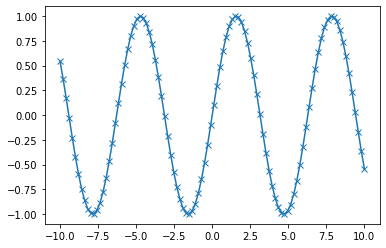
plot() is the main function to generate a plot (but many more exist):

plot(x, y)        Plot x vs y, default settings
plot(x, y, 'bo')  Plot x vs y, blue circle markers
plot(y, 'r+')     Plot y (x = array 0..N-1), red plusses

Every plotting function is completely customizable through a large set of options.

x = np.linspace(-10, 10, 100) # Sequence for X-axis 
y = np.sin(x) # sine values 
p = plt.plot(x, y, marker="x") # Line plot with marker x

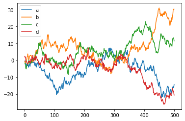
pandas + matplotlib

pandas DataFrames offer an easier, higher-level interface for matplotlib functions

df = pd.DataFrame(np.random.randn(500, 4), 
                  columns=['a', 'b', 'c', 'd']) # random 4D data
p = df.cumsum() # Plot cumulative sum of all series
p.plot();

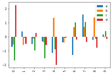
p = df[:10].plot(kind='bar') # First 10 arrays as bar plots  

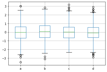
p = df.boxplot() # Boxplot for each of the 4 series

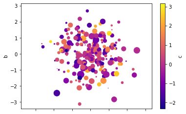
# Scatter plot using the 4 series for x, y, color, scale 
df.plot(kind='scatter', x='a', y='b', c='c', s=df['d']*72, cmap='plasma');

Advanced plotting libraries

Several libraries, such as Seaborn offer more advanced plots and easier interfaces.

Further reading links

• Matplotlib examples

• Plotting with pandas

• Seaborn examples