Lecture 3: Kernelization

Lecture 3: Kernelization#

Making linear models non-linear

Joaquin Vanschoren

Feature Maps#

Linear models: $\hat{y} = \mathbf{w}\mathbf{x} + w_0 = \sum_{i=1}^{p} w_i x_i + w_0 = w_0 + w_1 x_1 + ... + w_p x_p $
When we cannot fit the data well, we can add non-linear transformations of the features
Feature map (or basis expansion ) $\phi$ : $ X \rightarrow \mathbb{R}^d $

\[y=\textbf{w}^T\textbf{x} \rightarrow y=\textbf{w}^T\phi(\textbf{x})\]

E.g. Polynomial feature map: all polynomials up to degree $d$ and all products

\[[1, x_1, ..., x_p] \xrightarrow{\phi} [1, x_1, ..., x_p, x_1^2, ..., x_p^2, ..., x_p^d, x_1 x_2, ..., x_{p-1} x_p]\]

Example with $p=1, d=3$ :

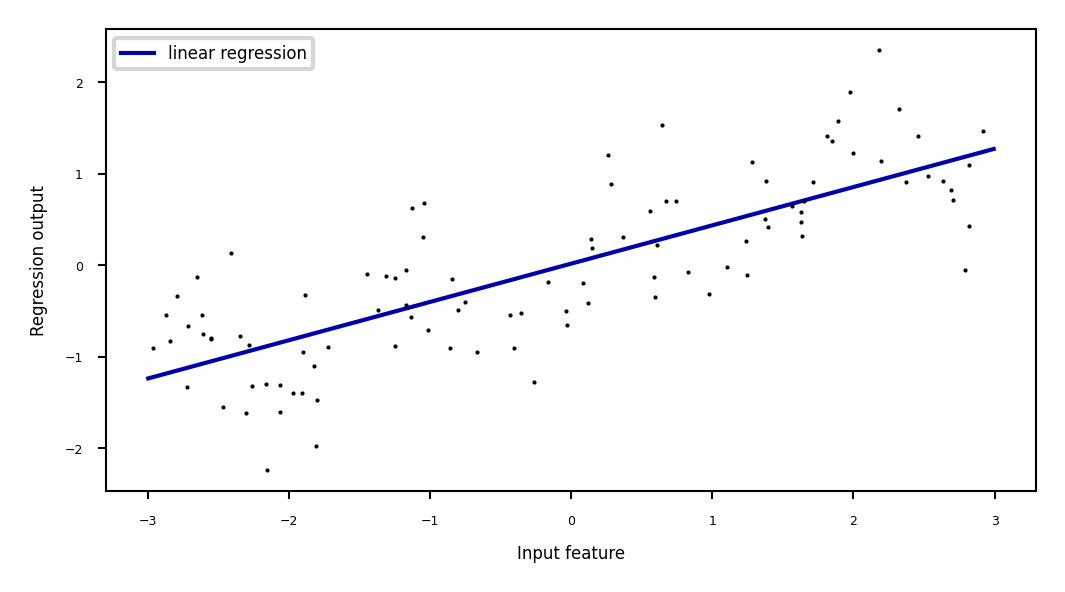
\[y=w_0 + w_1 x_1 \xrightarrow{\phi} y=w_0 + w_1 x_1 + w_2 x_1^2 + w_3 x_1^3\]

Ridge regression example#

Weights: [0.418]

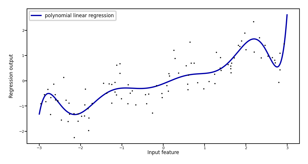
../_images/e9e8ed205fab1af77d9ec7a2c0cbd6c7926a17791cfeb8c5578bc112b6c72131.png

Add all polynomials $x^d$ up to degree 10 and fit again:
- e.g. use sklearn PolynomialFeatures

	x0	x0^2	x0^3	x0^4	x0^5	x0^6	x0^7	x0^8	x0^9	x0^10
0	-0.752759	0.566647	-0.426548	0.321088	-0.241702	0.181944	-0.136960	0.103098	-0.077608	0.058420
1	2.704286	7.313162	19.776880	53.482337	144.631526	391.124988	1057.713767	2860.360362	7735.232021	20918.278410
2	1.391964	1.937563	2.697017	3.754150	5.225640	7.273901	10.125005	14.093639	19.617834	27.307312
3	0.591951	0.350406	0.207423	0.122784	0.072682	0.043024	0.025468	0.015076	0.008924	0.005283
4	-2.063888	4.259634	-8.791409	18.144485	-37.448187	77.288869	-159.515582	329.222321	-679.478050	1402.366700

Weights: [ 0.643  0.297 -0.69  -0.264  0.41   0.096 -0.076 -0.014  0.004  0.001]

../_images/f57372c211a25d993921ecabb26d4703d1cd0b6567af87c772f35d8af99f79eb.png

How expensive is this?#

You may need MANY dimensions to fit the data
- Memory and computational cost
- More weights to learn, more likely overfitting
Ridge has a closed-form solution which we can compute with linear algebra: $$w^{*} = (X^{T}X + \alpha I)^{-1} X^T Y$$
Since X has $n$ rows (examples), and $d$ columns (features), $X^{T}X$ has dimensionality $d x d$
Hence Ridge is quadratic in the number of features, $\mathcal{O}(d^2n)$
After the feature map $\Phi$, we get $$w^{*} = (\Phi(X)^{T}\Phi(X) + \alpha I)^{-1} \Phi(X)^T Y$$
Since $\Phi$ increases $d$ a lot, $\Phi(X)^{T}\Phi(X)$ becomes huge

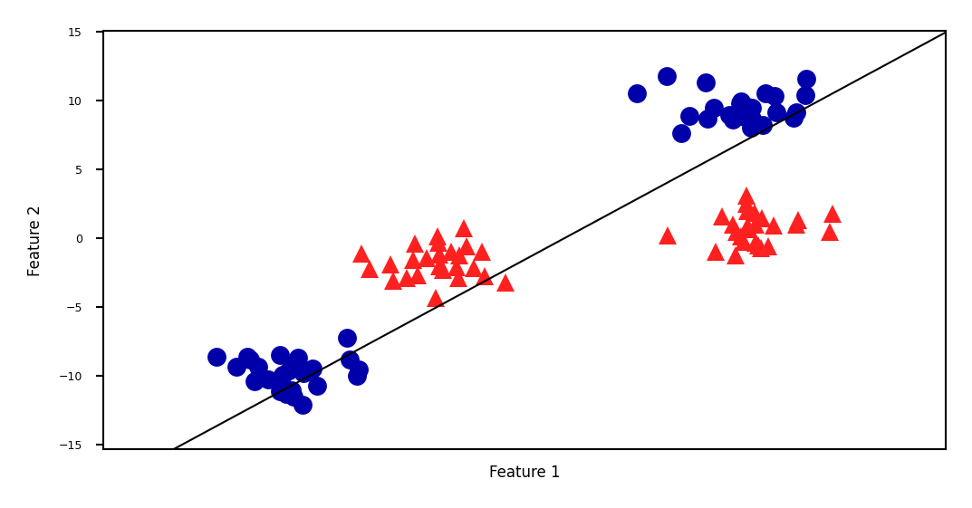
Linear SVM example (classification)#

../_images/1b770a0e5975b7d6810d5390cb0a2e9796058fad8dc21f79775ff600c355535d.png

We can add a new feature by taking the squares of feature1 values

../_images/4db8f8a1eb0dca18cbb47fce4f5d591dee6358169e2adfbbcf32882ca754901c.png

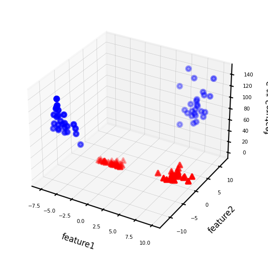
Now we can fit a linear model

../_images/acc7370c99ee266dbcea7f20e7e020d0e3d6d0252a726ab0ff2a31b164222aa9.png

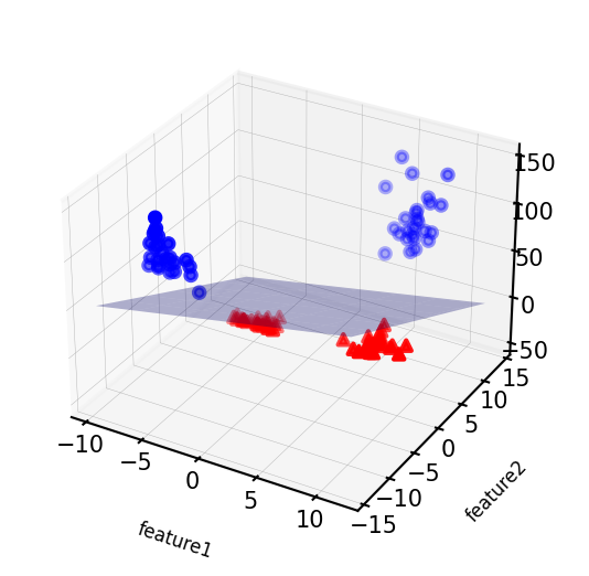
As a function of the original features, the decision boundary is now a polynomial as well $$y = w_0 + w_1 x_1 + w_2 x_2 + w_3 x_2^2 > 0$$

../_images/f809e2efb1820e732a106c19c0bafdff87b6f469b99816305862cdc465e98683.png

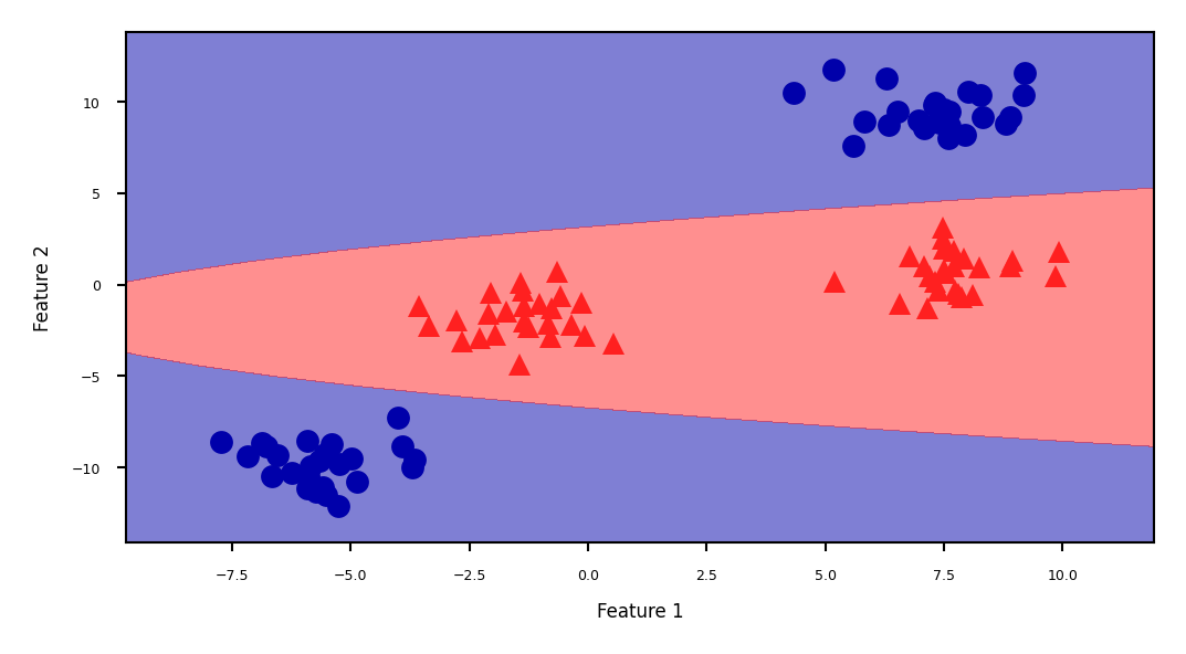
The kernel trick#

Computations in explicit, high-dimensional feature maps are expensive
For some feature maps, we can, however, compute distances between points cheaply
- Without explicitly constructing the high-dimensional space at all
Example: quadratic feature map for $\mathbf{x} = (x_1,..., x_p )$:

\[ \Phi(\mathbf{x}) = (x_1,..., x_p , x_1^2,..., x_p^2 , \sqrt{2} x_1 x_2 , ..., \sqrt{2} x_{p-1} x_{p}) \]

A kernel function exists for this feature map to compute dot products

\[ k_{quad}(\mathbf{x_i},\mathbf{x_j}) = \Phi(\mathbf{x_i}) \cdot \Phi(\mathbf{x_j}) = \mathbf{x_i} \cdot \mathbf{x_j} + (\mathbf{x_i} \cdot \mathbf{x_j})^2\]

Skip computation of $\Phi(x_i)$ and $\Phi(x_j)$ and compute $k(x_i,x_j)$ directly

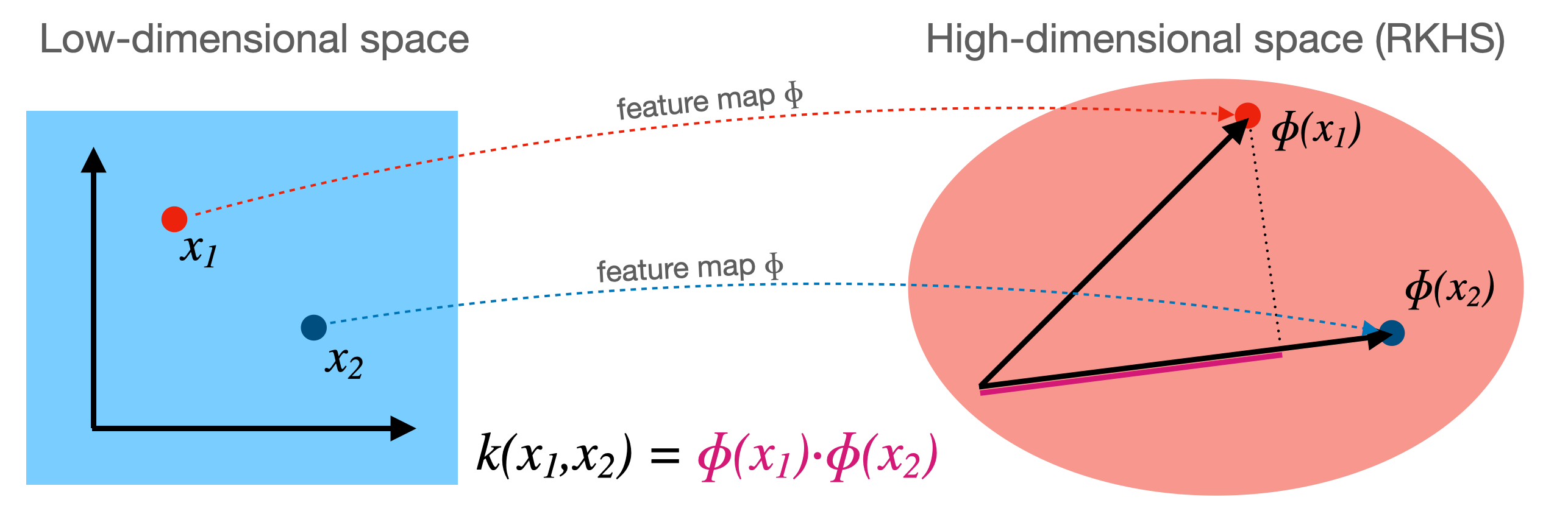
Kernelization#

Kernel $k$ corresponding to a feature map $\Phi$: $ k(\mathbf{x_i},\mathbf{x_j}) = \Phi(\mathbf{x_i}) \cdot \Phi(\mathbf{x_j})$
Computes dot product between $x_i,x_j$ in a high-dimensional space $\mathcal{H}$
- Kernels are sometimes called generalized dot products
- $\mathcal{H}$ is called the reproducing kernel Hilbert space (RKHS)
The dot product is a measure of the similarity between $x_i,x_j$
- Hence, a kernel can be seen as a similarity measure for high-dimensional spaces
If we have a loss function based on dot products $\mathbf{x_i}\cdot\mathbf{x_j}$ it can be kernelized
- Simply replace the dot products with $k(\mathbf{x_i},\mathbf{x_j})$

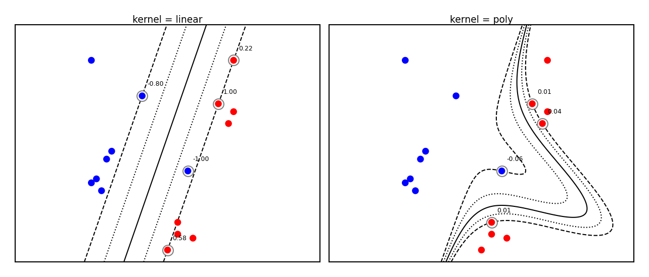
Example: SVMs#

Linear SVMs (dual form, for $l$ support vectors with dual coefficients $a_i$ and classes $y_i$): $$\mathcal{L}_{Dual} (a_i) = \sum_{i=1}^{l} a_i - \frac{1}{2} \sum_{i,j=1}^{l} a_i a_j y_i y_j (\mathbf{x_i} . \mathbf{x_j}) $$
Kernelized SVM, using any existing kernel $k$ we want: $$\mathcal{L}_{Dual} (a_i, k) = \sum_{i=1}^{l} a_i - \frac{1}{2} \sum_{i,j=1}^{l} a_i a_j y_i y_j k(\mathbf{x_i},\mathbf{x_j}) $$

Show code cell source Hide code cell source

from sklearn import svm

def plot_svm_kernels(kernels, poly_degree=3, gamma=2, C=1, size=4):
    # Our dataset and targets
    X = np.c_[(.4, -.7),
              (-1.5, -1),
              (-1.4, -.9),
              (-1.3, -1.2),
              (-1.1, -.2),
              (-1.2, -.4),
              (-.5, 1.2),
              (-1.5, 2.1),
              (1, 1),
              # --
              (1.3, .8),
              (1.2, .5),
              (.2, -2),
              (.5, -2.4),
              (.2, -2.3),
              (0, -2.7),
              (1.3, 2.1)].T
    Y = [0] * 8 + [1] * 8

    # figure number
    fig, axes = plt.subplots(-(-len(kernels)//3), min(len(kernels),3), figsize=(min(len(kernels),3)*size*1.2*fig_scale, -(-len(kernels)//3)*size*fig_scale), tight_layout=True)
    if len(kernels) == 1:
        axes = np.array([axes])
    if not isinstance(gamma,list):
        gamma = [gamma]*len(kernels)
    if not isinstance(C,list):
        C = [C]*len(kernels)
    # fit the model
    for kernel, ax, g, c in zip(kernels,axes.reshape(-1),gamma,C):
        clf = svm.SVC(kernel=kernel, gamma=g, C=c, degree=poly_degree)
        clf.fit(X, Y)

        # plot the line, the points, and the nearest vectors to the plane
        if kernel == 'rbf':
            ax.set_title(r"kernel = {}, $\gamma$={}, C={}".format(kernel, g, c), pad=0.1)
        else:
            ax.set_title('kernel = %s' % kernel,pad=0.1)

        ax.scatter(clf.support_vectors_[:, 0], clf.support_vectors_[:, 1],
                    s=25, edgecolors='grey', c='w', zorder=10, linewidths=0.5)
        ax.scatter(X[:, 0], X[:, 1], c=Y, zorder=10, cmap=plt.cm.bwr, s=10*fig_scale)

        for i, coef in enumerate(clf.dual_coef_[0]):
            ax.annotate("%0.2f" % (coef), (clf.support_vectors_[i, 0]+0.1,clf.support_vectors_[i, 1]+0.25), zorder=11, fontsize=3)

        ax.axis('tight')
        x_min = -3
        x_max = 3
        y_min = -3
        y_max = 3

        XX, YY = np.mgrid[x_min:x_max:200j, y_min:y_max:200j]
        Z = clf.decision_function(np.c_[XX.ravel(), YY.ravel()])

        # Put the result into a color plot
        Z = Z.reshape(XX.shape)
        #plt.pcolormesh(XX, YY, Z > 0, cmap=plt.cm.bwr, alpha=0.1)
        ax.contour(XX, YY, Z, colors=['k', 'k', 'k', 'k', 'k'], linestyles=['--', ':', '-', ':', '--'],
                    levels=[-1, -0.5, 0, 0.5, 1])

        ax.set_xlim(x_min, x_max)
        ax.set_ylim(y_min, y_max)

        ax.set_xticks([])
        ax.set_yticks([])

    plt.tight_layout()
    plt.show()
plot_svm_kernels(['linear', 'poly'],poly_degree=3,size=3.5)

../_images/742b04a10cbb0f2eea7621b2d0ff646cc1409f3ccafb72432a5d88d4e13d592e.png

Which kernels exist?#

A (Mercer) kernel is any function $k: X \times X \rightarrow \mathbb{R}$ with these properties:
- Symmetry: $k(\mathbf{x_1},\mathbf{x_2}) = k(\mathbf{x_2},\mathbf{x_1}) \,\,\, \forall \mathbf{x_1},\mathbf{x_2} \in X$
- Positive definite: the kernel matrix $K$ is positive semi-definite
  - Intuitively, $k(\mathbf{x_1},\mathbf{x_2}) \geq 0$
The kernel matrix (or Gram matrix) for $n$ points of $x_1,..., x_n \in X$ is defined as:

\[\begin{split} K = XX^T = \begin{bmatrix} k(\mathbf{x_1}, \mathbf{x_1}) & \ldots & k(\mathbf{x_1}, \mathbf{x_n}) \\ \vdots & \ddots & \vdots \\ k(\mathbf{x_n}, \mathbf{x_1}) & \ldots & k(\mathbf{x_n}, \mathbf{x_n}) \end{bmatrix} \end{split}\]

Once computed ($\mathcal{O}(n^2)$), simply lookup $k(\mathbf{x_1}, \mathbf{x_2})$ for any two points
In practice, you can either supply a kernel function or precompute the kernel matrix

Linear kernel#

Input space is same as output space: $X = \mathcal{H} = \mathbb{R}^d$
Feature map $\Phi(\mathbf{x}) = \mathbf{x}$
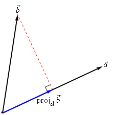
Kernel: $ k_{linear}(\mathbf{x_i},\mathbf{x_j}) = \mathbf{x_i} \cdot \mathbf{x_j}$
Geometrically, the dot product is the projection of $\mathbf{x_j}$ on hyperplane defined by $\mathbf{x_i}$
- Becomes larger if $\mathbf{x_i}$ and $\mathbf{x_j}$ are in the same ‘direction’

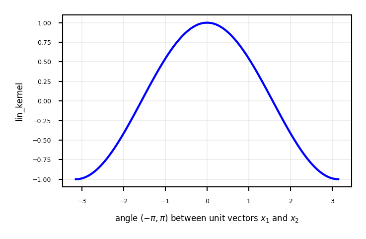
Linear kernel between point (0,1) and another unit vector an angle $a$ (in radians)
- Points with similar angles are deemed similar

../_images/6bd01c2f71829d1d80c55876ded6a54722185daa6d4caf3b3f70cdee7d26c3db.png

Polynomial kernel#

If $k_1$, $k_2$ are kernels, then $\lambda . k_1$ ($\lambda \geq 0$), $k_1 + k_2$, and $k_1 . k_2$ are also kernels
The polynomial kernel (for degree $d \in \mathbb{N}$) reproduces the polynomial feature map
- $\gamma$ is a scaling hyperparameter (default $\frac{1}{p}$)
- $c_0$ is a hyperparameter (default 1) to trade off influence of higher-order terms $$k_{poly}(\mathbf{x_1},\mathbf{x_2}) = (\gamma (\mathbf{x_1} \cdot \mathbf{x_2}) + c_0)^d$$

RBF (Gaussian) kernel#

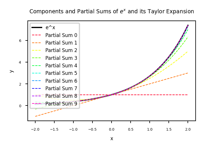
The Radial Basis Function (RBF) feature map is related to the Taylor series expansion of $e^x$ $$\Phi(x) = e^{-x^2/2\gamma^2} \Big[ 1, \sqrt{\frac{1}{1!\gamma^2}}x,\sqrt{\frac{1}{2!\gamma^4}}x^2,\sqrt{\frac{1}{3!\gamma^6}}x^3,\ldots\Big]^T$$
RBF (or Gaussian ) kernel with kernel width $\gamma \geq 0$:
$$k_{RBF}(\mathbf{x_1},\mathbf{x_2}) = exp(-\gamma ||\mathbf{x_1} - \mathbf{x_2}||^2)$$

Taylor expansion: the more we add components, the more we can approximate any function

import matplotlib.cm as cm

# Generate x values
x = np.linspace(-2, 2, 100)

# Calculate corresponding y values for e^x
y_actual = np.exp(x)

# Plot the actual function
fig, ax = plt.subplots(figsize=(5*fig_scale,3*fig_scale))
plt.plot(x, y_actual, label='e^x', linewidth=1, color='black')

# Plot the individual terms of the Taylor expansion with formulas in the legend
colors = cm.gist_rainbow(np.linspace(0, 1, 10))  # Color scheme from red to blue
for n in range(10):
    term = x**n / np.math.factorial(n)
    partial_sum = np.sum([x**i / np.math.factorial(i) for i in range(n + 1)], axis=0)
    
    # Plot partial sums with different colors
    plt.plot(x, partial_sum, label=f'Partial Sum {n}', linestyle='dashed', color=colors[n])

# Add labels and title
plt.xlabel('x')
plt.ylabel('y')
plt.title('Components and Partial Sums of $e^x$ and its Taylor Expansion')

# Display legend
plt.legend();

../_images/a3eef376fb4c7e69f7225346f5386bfb62becbd2576de13b4eadec31973a7c76.png

The RBF kernel $k_{RBF}(\mathbf{x_1},\mathbf{x_2}) = exp(-\gamma ||\mathbf{x_1} - \mathbf{x_2}||^2)$ does not use a dot product
- It only considers the distance between $\mathbf{x_1}$ and $\mathbf{x_2}$
- It’s a local kernel : every data point only influences data points nearby
  - linear and polynomial kernels are global : every point affects the whole space
- Similarity depends on closeness of points and kernel width
  - value goes up for closer points and wider kernels (larger overlap)

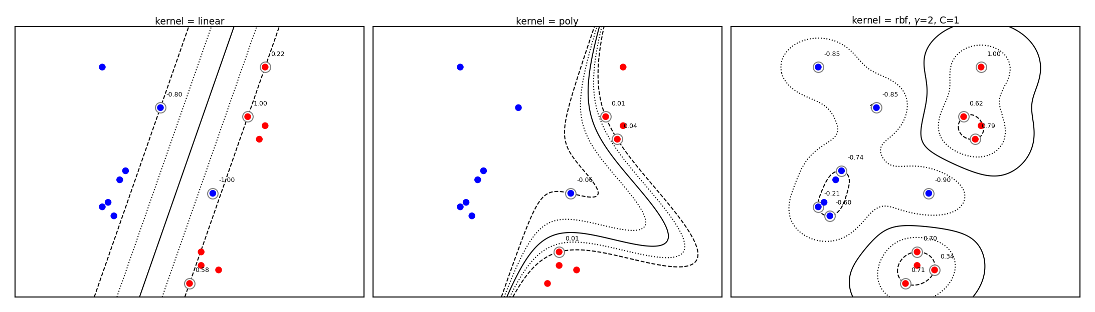
Kernelized SVMs in practice#

You can use SVMs with any kernel to learn non-linear decision boundaries

../_images/7f914595786f7fe0f588a822959629df7fbb372ec727476b4cfca8f4788683a6.png

SVM with RBF kernel#

Every support vector locally influences predictions, according to kernel width ($\gamma$)
The prediction for test point $\mathbf{u}$: sum of the remaining influence of each support vector
- $f(x) = \sum_{i=1}^{l} a_i y_i k(\mathbf{x_i},\mathbf{u})$

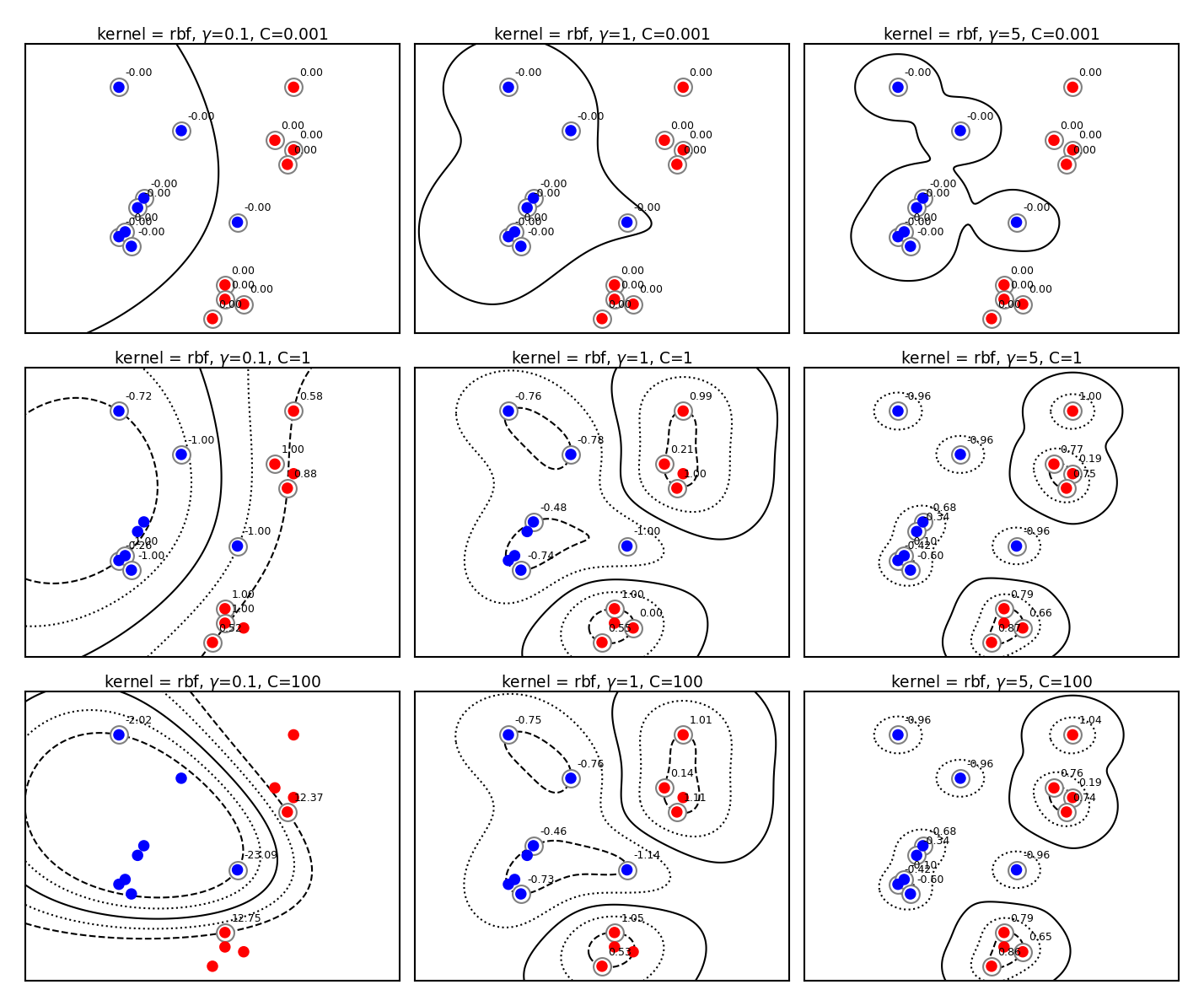
Tuning RBF SVMs#

gamma (kernel width)
- high values cause narrow Gaussians, more support vectors, overfitting
- low values cause wide Gaussians, underfitting
C (cost of margin violations)
- high values punish margin violations, cause narrow margins, overfitting
- low values cause wider margins, more support vectors, underfitting

../_images/e17e93993151cb09f4f4af72b8aa796ea4d2fb4690213222346f4e75e97af2a3.png

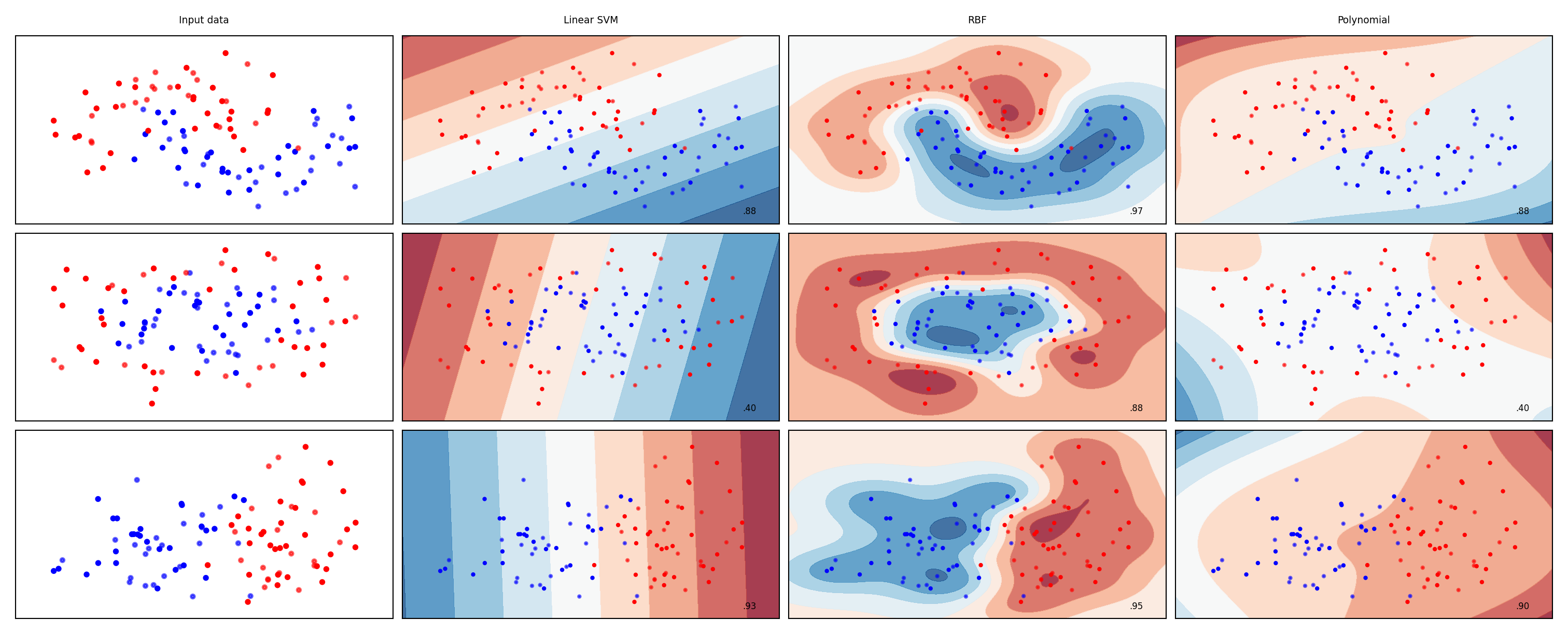
Kernel overview

../_images/5a3fe7e89fe2f6cccd663d3986301149ab6688529a30d9ada791c233f6f56080.png

SVMs in practice#

C and gamma always need to be tuned
- Interacting regularizers. Find a good C, then finetune gamma
SVMs expect all features to be approximately on the same scale
- Data needs to be scaled beforehand
Allow to learn complex decision boundaries, even with few features
- Work well on both low- and high dimensional data
- Especially good at small, high-dimensional data
Hard to inspect, although support vectors can be inspected
In sklearn, you can use SVC for classification with a range of kernels
- SVR for regression

Other kernels#

There are many more possible kernels
If no kernel function exists, we can still precompute the kernel matrix
- All you need is some similarity measure, and you can use SVMs
Text kernels:
- Word kernels: build a bag-of-words representation of the text (e.g. TFIDF)
  - Kernel is the inner product between these vectors
- Subsequence kernels: sequences are similar if they share many sub-sequences
  - Build a kernel matrix based on pairwise similarities
Graph kernels: Same idea (e.g. find common subgraphs to measure similarity)
These days, deep learning embeddings are more frequently used

The Representer Theorem#

We can kernelize many other loss functions as well
The Representer Theorem states that if we have a loss function $\mathcal{L}'$ with
- $\mathcal{L}$ an arbitrary loss function using some function $f$ of the inputs $\mathbf{x}$
- $\mathcal{R}$ a (non-decreasing) regularization score (e.g. L1 or L2) and constant $\lambda$ $$\mathcal{\mathcal{L}'}(\mathbf{w}) = \mathcal{L}(y,f(\mathbf{x})) + \lambda \mathcal{R} (||\mathbf{w}||)$$
Then the weights $\mathbf{w}$ can be described as a linear combination of the training samples: $$\mathbf{w} = \sum_{i=1}^{n} a_i y_i f(\mathbf{x_i})$$
Note that this is exactly what we found for SVMs: $ \mathbf{w} = \sum_{i=1}^{l} a_i y_i \mathbf{\mathbf{x_i}} $
Hence, we can also kernelize Ridge regression, Logistic regression, Perceptrons, Support Vector Regression, …

Kernelized Ridge regression#

The linear Ridge regression loss (with $\mathbf{x_0}=1$): $$\mathcal{L}_{Ridge}(\mathbf{w}) = \sum_{i=0}^{n} (y_i-\mathbf{w}\mathbf{x_i})^2 + \lambda \| w \|^2$$
Filling in $\mathbf{w} = \sum_{i=1}^{n} \alpha_i y_i \mathbf{x_i}$ yields the dual formulation: $$\mathcal{L}_{Ridge}(\mathbf{w}) = \sum_{i=1}^{n} (y_i-\sum_{j=1}^{n} \alpha_j y_j \mathbf{x_i}\mathbf{x_j})^2 + \lambda \sum_{i=1}^{n} \sum_{j=1}^{n} \alpha_i \alpha_j y_i y_j \mathbf{x_i}\mathbf{x_j}$$
Generalize $\mathbf{x_i}\cdot\mathbf{x_j}$ to $k(\mathbf{x_i},\mathbf{x_j})$ $$\mathcal{L}_{KernelRidge}(\mathbf{\alpha},k) = \sum_{i=1}^{n} (y_i-\sum_{j=1}^{n} \alpha_j y_j k(\mathbf{x_i},\mathbf{x_n}))^2 + \lambda \sum_{i=1}^{n} \sum_{j=1}^{n} \alpha_i \alpha_j y_i y_j k(\mathbf{x_i},\mathbf{x_j})$$

Example of kernelized Ridge#

Prediction (red) is now a linear combination of kernels (blue): $y = \sum_{j=1}^{n} \alpha_j y_j k(\mathbf{x},\mathbf{x_j})$
We learn a dual coefficient for each point

Fitting our regression data with KernelRidge

Other kernelized methods#

Same procedure can be done for logistic regression
For perceptrons, $\alpha \rightarrow \alpha+1$ after every misclassification $$\mathcal{L}_{DualPerceptron}(x_i,k) = max(0,y_i \sum_{j=1}^{n} \alpha_j y_j k(\mathbf{x_j},\mathbf{x_i}))$$
Support Vector Regression behaves similarly to Kernel Ridge

Summary#

Feature maps $\Phi(x)$ transform features to create a higher-dimensional space
- Allows learning non-linear functions or boundaries, but very expensive/slow
For some $\Phi(x)$, we can compute dot products without constructing this space
- Kernel trick: $k(\mathbf{x_i},\mathbf{x_j}) = \Phi(\mathbf{x_i}) \cdot \Phi(\mathbf{x_j})$
- Kernel $k$ (generalized dot product) is a measure of similarity between $\mathbf{x_i}$ and $\mathbf{x_j}$
There are many such kernels
- Polynomial kernel: $k_{poly}(\mathbf{x_1},\mathbf{x_2}) = (\gamma (\mathbf{x_1} \cdot \mathbf{x_2}) + c_0)^d$
- RBF (Gaussian) kernel: $k_{RBF}(\mathbf{x_1},\mathbf{x_2}) = exp(-\gamma ||\mathbf{x_1} - \mathbf{x_2}||^2)$
- A kernel matrix can be precomputed using any similarity measure (e.g. for text, graphs,…)
Any loss function where inputs appear only as dot products can be kernelized
- E.g. Linear SVMs: simply replace the dot product with a kernel of choice
The Representer theorem states which other loss functions can also be kernelized and how
- Ridge regression, Logistic regression, Perceptrons,…