
Lab 7a: Convolutional neural nets#
In this lab we consider the CIFAR dataset, but model it using convolutional neural networks instead of linear models. There is no separate tutorial, but you can find lots of examples in the lecture notebook on convolutional neural networks. If you are very confident, you can also try to solve these exercises using PyTorch instead of TensorFlow.
Tip: You can run these exercises faster on a GPU (but they will also run fine on a CPU). If you do not have a GPU locally, you can upload this notebook to Google Colab. You can enable GPU support at “runtime” -> “change runtime type”.
# Auto-setup when running on Google Colab
if 'google.colab' in str(get_ipython()):
    !pip install openml

# General imports
%matplotlib inline
import numpy as np
import pandas as pd
import matplotlib.pyplot as plt
import openml as oml
import tensorflow as tf
# Uncomment the next line if you run on Colab
#!pip install --quiet openml
%matplotlib inline
import openml as oml
import matplotlib.pyplot as plt
# Download CIFAR data. Takes a while the first time.
# This version returns 3x32x32 resolution images.
# If you feel like it, repeat the exercises with the 96x96x3 resolution version by using ID 41103
cifar = oml.datasets.get_dataset(40926)
X, y, _, _ = cifar.get_data(target=cifar.default_target_attribute, dataset_format='array');
cifar_classes = {0: "airplane", 1: "automobile", 2: "bird", 3: "cat", 4: "deer",
                 5: "dog", 6: "frog", 7: "horse", 8: "ship", 9: "truck"}
# The dataset (40926) is in a weird 3x32x32 format, we need to reshape and transpose
Xr = X.reshape((len(X),3,32,32)).transpose(0,2,3,1)
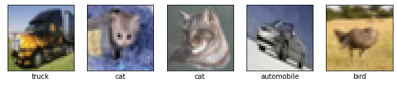
# Take some random examples, reshape to a 32x32 image and plot
from random import randint
fig, axes = plt.subplots(1, 5,  figsize=(10, 5))
for i in range(5):
    n = randint(0,len(Xr))
    # The data is stored in a 3x32x32 format, so we need to transpose it
    axes[i].imshow(Xr[n]/255)
    axes[i].set_xlabel((cifar_classes[int(y[n])]))
    axes[i].set_xticks(()), axes[i].set_yticks(())
plt.show();
Exercise 1: A simple model#
Split the data into 80% training and 20% validation sets
Normalize the data to [0,1]
Build a ConvNet with 3 convolutional layers interspersed with MaxPooling layers, and one dense layer.
Use at least 32 3x3 filters in the first layer and ReLU activation.
Otherwise, make rational design choices or experiment a bit to see what works.
You should at least get 60% accuracy.
For training, you can try batch sizes of 64, and 20-50 epochs, but feel free to explore this as well
Plot and interpret the learning curves. Is the model overfitting? How could you improve it further?
Exercise 2: VGG-like model#
Implement a simplified VGG model by building 3 ‘blocks’ of 2 convolutional layers each
Do MaxPooling after each block
The first block should use at least 32 filters, later blocks should use more
You can use 3x3 filters
Use zero-padding to be able to build a deeper model (see the
paddingattribute)Use a dense layer with at least 128 hidden nodes.
You can use ReLU activations everywhere (where it makes sense)
Plot and interpret the learning curves
Exercise 3: Regularization#
Explore different ways to regularize your VGG-like model
Try adding some dropout after every MaxPooling and Dense layer.
What are good Dropout rates? Try a fixed Dropout rate, or increase the rates in the deeper layers.
Try batch normalization together with Dropout
Think about where batch normalization would make sense
Plot and interpret the learning curves
Exercise 4: Data Augmentation#
Perform image augmentation (rotation, shift, shear, zoom, flip,…). You can use the ImageDataGenerator for this.
What is the effect? What is the effect with and without Dropout?
Plot and interpret the learning curves
Exercise 5: Interpret the misclassifications#
Chances are that even your best model is not yet perfect. It is important to understand what kind of errors it still makes.
Run the test images through the network and detect all misclassified ones
Interpret some of the misclassifications. Are these misclassifications to be expected?
Compute the confusion matrix. Which classes are often confused?
Exercise 6: Interpret the model#
Retrain your best model on all the data. Next, retrieve and visualize the activations (feature maps) for every filter for every convolutional layer, or at least for a few filters for every layer. Tip: see the course notebooks for examples on how to do this.
Interpret the results. Is your model indeed learning something useful?
Optional: Take it a step further#
Repeat the exercises, but now use a higher-resolution version of the CIFAR dataset (with OpenML ID 41103), or another version with 100 classes (with OpenML ID 41983). Good luck!