
Recap: Decision Trees#
Representation: Assume we can represent the concept we want to learn with a decision tree
Repeatedly split the data based on one feature at a time
Note: Oblique trees can split on combinations of features
Evaluation (loss): One tree is better that another tree according to some heuristic
Classification: Instances in a leaf are mostly of the same class (
pureleafs)Regression: Instances in a leaf have values close to each other
Optimization: Recursive, heuristic greedy search (Hunt’s algorithm)
Make first split based on the heuristic
In each branch, repeat splitting in the same way
# Auto-setup when running on Google Colab
import os
if 'google.colab' in str(get_ipython()) and not os.path.exists('/content/master'):
    !git clone -q https://github.com/ML-course/master.git /content/master
    !pip install -rq master/requirements_colab.txt
    %cd master/notebooks

# Global imports and settings
%matplotlib inline
from preamble import *
interactive = True # Set to True for interactive plots
if interactive:
    fig_scale = 1.5
Installation note#
To plot the decision trees in this notebook, you’ll need to install the graphviz executable:
OS X: use homebrew:
brew install graphvizUbuntu/debian: use apt-get:
apt-get install graphviz.Installing graphviz on Windows can be tricky and using conda / anaconda is recommended.
And the python package: pip install graphviz
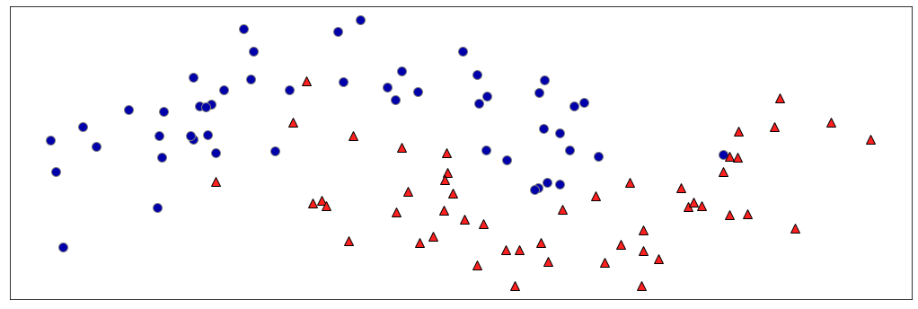
Decision Tree classification#
Where would you make the first split?
from sklearn.tree import DecisionTreeClassifier
from sklearn.datasets import make_moons

X, y = make_moons(n_samples=100, noise=0.25, random_state=3)
plt.figure(figsize=(12*fig_scale,4*fig_scale))
ax = plt.gca()
mglearn.tools.discrete_scatter(X[:, 0], X[:, 1], y, ax=ax)
ax.set_xticks(())
ax.set_yticks(());
import graphviz
def plot_depth(depth):
fig, ax = plt.subplots(1, 2, figsize=(12*fig_scale, 4*fig_scale),
subplot_kw={'xticks': (), 'yticks': ()})
tree = mglearn.plots.plot_tree(X, y, max_depth=depth)
ax[0].imshow(mglearn.plots.tree_image(tree))
ax[0].set_axis_off()
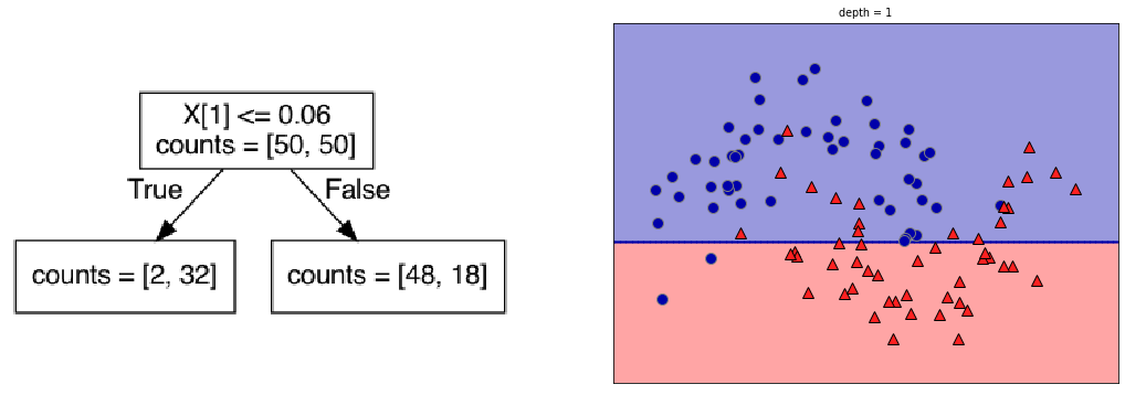
plot_depth(1)
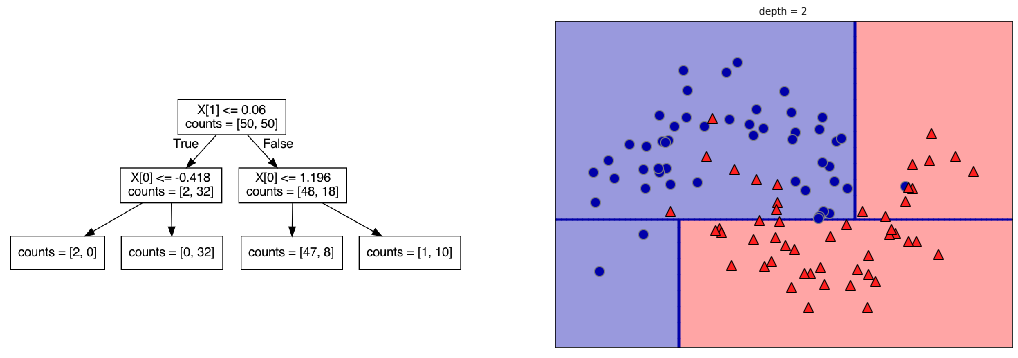
plot_depth(2)
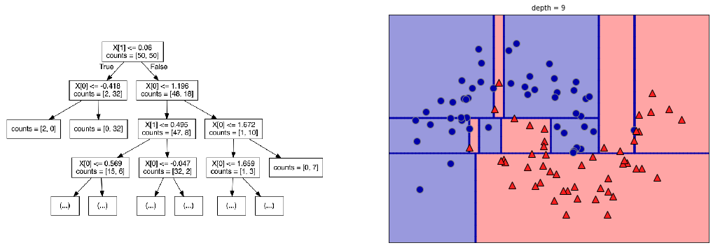
plot_depth(9)
Heuristics#
We start from a dataset of \(n\) points \(D = \{(x_i,y_i)\}_{i=1}^{n}\) where \(y_i\) is one of \(k\) classes
Consider splits between adjacent data point of different class, for every variable
After splitting, each leaf will have \(\hat{p}_k\) = the relative frequency of class \(k\)
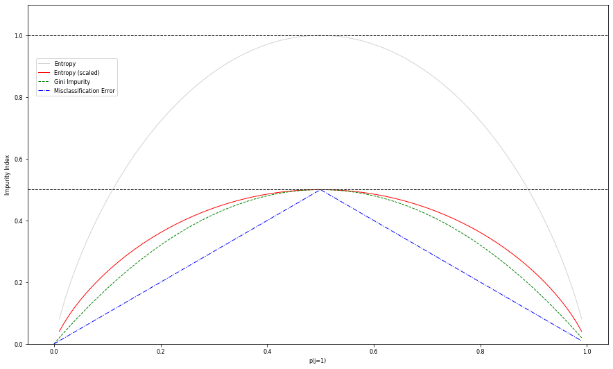
We can define several impurity measures:
Misclassification Error (leads to larger trees): \( 1 - \underset{k}{\operatorname{argmax}} \hat{p}_{k} \)
Gini-Index: \( \sum_{k\neq k'} \hat{p}_k \hat{p}_{k'} = \sum_{k=1}^K \hat{p}_k(1-\hat{p}_k) \)
Sum up the heuristics per leaf, weighted by the number of examples in each leaf
Visualization: the plots on the right show the class distribution of the ‘top’ and ‘bottom’ leaf, respectively.
from __future__ import print_function
import ipywidgets as widgets
from ipywidgets import interact, interact_manual

def misclassification_error(leaf1_distr, leaf2_distr, leaf1_size, leaf2_size):
    total = leaf1_size + leaf2_size
    return leaf1_size/total * (1 - max(leaf1_distr)) + leaf2_size/total * (1 - max(leaf2_distr))

def gini_index(leaf1_distr, leaf2_distr, leaf1_size, leaf2_size):
    total = leaf1_size + leaf2_size
    return leaf1_size/total * np.array([leaf1_distr[k]*(1-leaf1_distr[k]) for k in range(0,2)]).sum() + \
            leaf2_size/total * np.array([leaf2_distr[k]*(1-leaf2_distr[k]) for k in range(0,2)]).sum()

@interact
def plot_heuristics(split=(-0.5,1.5,0.05)):

    fig, ax = plt.subplots(1, 2, figsize=(12*fig_scale, 4*fig_scale),
                           subplot_kw={'xticks': (), 'yticks': ()})
    mglearn.tools.discrete_scatter(X[:, 0], X[:, 1], y, ax=ax[0])
    ax[0].plot([min(X[:, 0]),max(X[:, 0])],[split,split])

    ind = np.arange(2)
    width = 0.35
    top, bottom = y[np.where(X[:, 1]>split)], y[np.where(X[:, 1]<=split)]
    top_0, top_1 = (top == 0).sum()/len(top), (top == 1).sum()/len(top)
    bottom_0, bottom_1 = (bottom == 0).sum()/len(bottom), (bottom == 1).sum()/len(bottom)
    ax[1].barh(ind, [bottom_1,top_1], width, color='r')
    for i, v in enumerate([bottom_1,top_1]):
        ax[1].text(0, i, 'p_1={:.2f}'.format(v), color='black', fontweight='bold')
    ax[1].barh(ind+width, [bottom_0,top_0], width, color='royalblue')
    for i, v in enumerate([bottom_0,top_0]):
        ax[1].text(0, i + width, 'p_0={:.2f}'.format(v), color='black', fontweight='bold')
    error = misclassification_error([top_0,top_1],[bottom_0,bottom_1],len(top),len(bottom))
    gini = gini_index([top_0,top_1],[bottom_0,bottom_1],len(top),len(bottom))
    ax[1].set_title("Misclass. Error:{:.2f}, Gini:{:.2f}".format(error, gini))
if not interactive:
    plot_heuristics(split=0.6)
Entropy (of the class attribute) measures unpredictability of the data:
How likely will random example have class k? $\( E(X) = -\sum_{k=1}^K \hat{p}_k \log_{2}\hat{p}_k \)$
Information Gain (a.k.a. Kullback–Leibler divergence) measures how much entropy has reduced by splitting on attribute \(X_i\): $\( G(X,X_i) = E(X) - \sum_{l=1}^L \frac{|X_{i=l}|}{|X_{i}|} E(X_{i=l}) \)$
with \(X\) = the training set, \(l\) a specific leaf after splitting on feature \(X_i\), \(X_{i=l}\) is the set of examples in leaf \(l\): \(\{x \in X | X_i \in l\}\)
Heuristics visualized (binary class)
Note that
gini != entropy/2
def gini(p):
   return (p)*(1 - (p)) + (1 - p)*(1 - (1-p))

def entropy(p):
   return - p*np.log2(p) - (1 - p)*np.log2((1 - p))

def classification_error(p):
   return 1 - np.max([p, 1 - p])

x = np.arange(0.0, 1.0, 0.01)
ent = [entropy(p) if p != 0 else None for p in x]
scaled_ent = [e*0.5 if e else None for e in ent]
c_err = [classification_error(i) for i in x]

fig = plt.figure(figsize=(10*fig_scale,6*fig_scale))
ax = plt.subplot(111)

for j, lab, ls, c, in zip(
      [ent, scaled_ent, gini(x), c_err],
      ['Entropy', 'Entropy (scaled)', 'Gini Impurity', 'Misclassification Error'],
      ['-', '-', '--', '-.'],
      ['lightgray', 'red', 'green', 'blue']):
   line = ax.plot(x, j, label=lab, linestyle=ls, lw=1, color=c)

ax.legend(loc='upper left', bbox_to_anchor=(0.01, 0.85),
         ncol=1, fancybox=True, shadow=False)
ax.axhline(y=0.5, linewidth=1, color='k', linestyle='--')
ax.axhline(y=1.0, linewidth=1, color='k', linestyle='--')

plt.ylim([0, 1.1])
plt.xlabel('p(j=1)')
plt.ylabel('Impurity Index')
plt.show()
%%HTML
<style>
td {font-size: 20px}
th {font-size: 20px}
.rendered_html table, .rendered_html td, .rendered_html th {
    font-size: 20px;
}
</style>
Example#
Compute information gain for a dataset with categorical features:
Ex. |
1 |
2 |
3 |
4 |
5 |
6 |
|---|---|---|---|---|---|---|
a1 |
T |
T |
T |
F |
F |
F |
a2 |
T |
T |
F |
F |
T |
T |
class |
+ |
+ |
- |
+ |
- |
- |
Ex. |
1 |
2 |
3 |
4 |
5 |
6 |
|---|---|---|---|---|---|---|
a1 |
T |
T |
T |
F |
F |
F |
a2 |
T |
T |
F |
F |
T |
T |
class |
+ |
+ |
- |
+ |
- |
- |
\(E(X)\) = \(-(\frac{1}{2}*log_2(\frac{1}{2})+\frac{1}{2}*log_2(\frac{1}{2})) = 1\) (classes have equal probabilities)
\(G(X, X_{a2})\) = 0 (after split, classes still have equal probabilities, entropy stays 1)
Ex. |
1 |
2 |
3 |
4 |
5 |
6 |
|---|---|---|---|---|---|---|
a1 |
T |
T |
T |
F |
F |
F |
a2 |
T |
T |
F |
F |
T |
T |
class |
+ |
+ |
- |
+ |
- |
- |
hence we split on a1
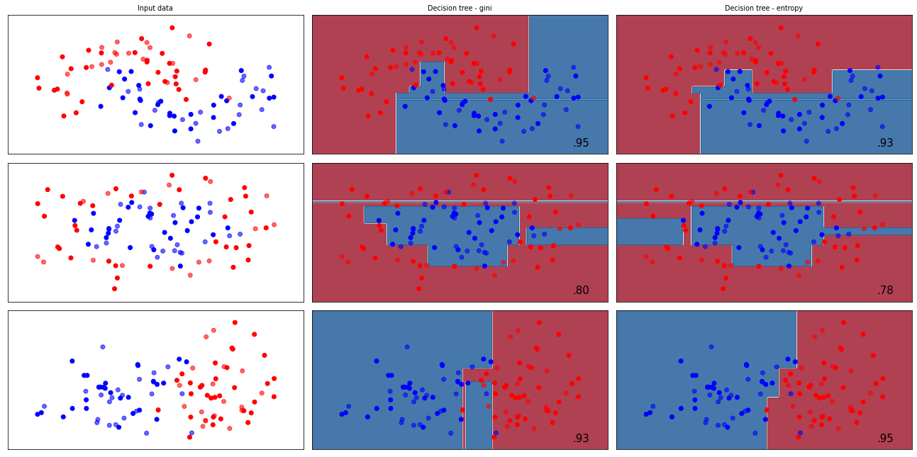
Heuristics in scikit-learn#
The splitting criterion can be set with the criterion option in DecisionTreeClassifier
gini(default): gini impurity indexentropy: information gain
Best value depends on dataset, as well as other hyperparameters
from sklearn.tree import DecisionTreeClassifier
names = ["Decision tree - gini", "Decision tree - entropy"]

classifiers = [
    DecisionTreeClassifier(),
    DecisionTreeClassifier(criterion="entropy")
    ]

mglearn.plots.plot_classifiers(names, classifiers, figuresize=(12*fig_scale,6*fig_scale))
Handling many-valued features#
What happens when a categorical feature has (almost) as many values as examples?
Information Gain will select it
One approach: use Gain Ratio instead (not available scikit-learn): $\( GainRatio(X,X_i) = \frac{Gain(X,X_i)}{SplitInfo(X,X_i)}\)\( \)\( SplitInfo(X,X_i) = - \sum_{v=1}^V \frac{|X_{i=v}|}{|X|} log_{2} \frac{|X_{i=v}|}{|X|} \)$
where \(X_{i=v}\) is the subset of examples for which feature \(X_i\) has value v.
SplitInfo will be big if \(X_i\) fragments the data into many small subsets, resulting in a smaller Gain Ratio.
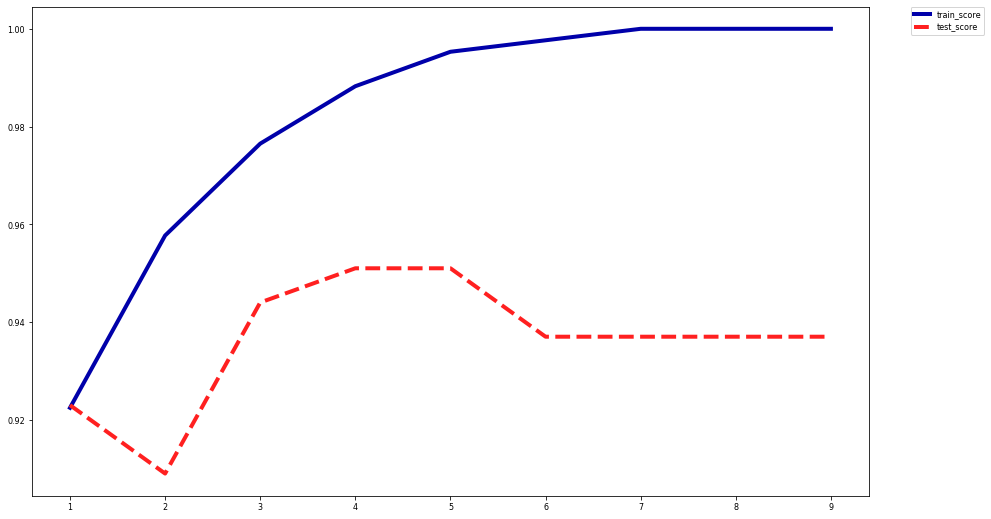
Overfitting: Controlling complexity of Decision Trees#
Decision trees can very easily overfit the data. Regularization strategies:
Pre-pruning: stop creation of new leafs at some point
Limiting the depth of the tree, or the number of leafs
Requiring a minimal leaf size (number of instances) to allow a split
Post-pruning: build full tree, then prune (join) leafs
Reduced error pruning: evaluate against held-out data
Many other strategies exist.
scikit-learn supports none of them (yet)
Effect of pre-pruning:
Shallow trees tend to underfit (high bias)
Deep trees tend to overfit (high variance)
from sklearn.datasets import load_breast_cancer
from sklearn.tree import DecisionTreeClassifier
from sklearn.model_selection import train_test_split

cancer = load_breast_cancer()
X_train, X_test, y_train, y_test = train_test_split(
    cancer.data, cancer.target, stratify=cancer.target, random_state=42)
train_score, test_score = [],[]
for depth in range(1,10):
    tree = DecisionTreeClassifier(random_state=0, max_depth=depth).fit(X_train, y_train)
    train_score.append(tree.score(X_train, y_train))
    test_score.append(tree.score(X_test, y_test))
plt.figure(figsize=(10*fig_scale,6*fig_scale))
plt.plot(range(1,10), train_score, label="train_score", linewidth=4)
plt.plot(range(1,10), test_score, label="test_score", linewidth=4)
plt.legend(bbox_to_anchor=(1.05, 1), loc='upper left', borderaxespad=0.)
<matplotlib.legend.Legend at 0x29c5f2580>
Decision Trees are easy to interpet
Visualize and find the path that most data takes
# Creates a .dot file
from sklearn.tree import export_graphviz
export_graphviz(tree, out_file="tree.dot", class_names=["malignant", "benign"],
                feature_names=cancer.feature_names, impurity=False, filled=True)
# Open and display
import graphviz
with open("tree.dot") as f:
    dot_graph = f.read()
display(graphviz.Source(dot_graph))

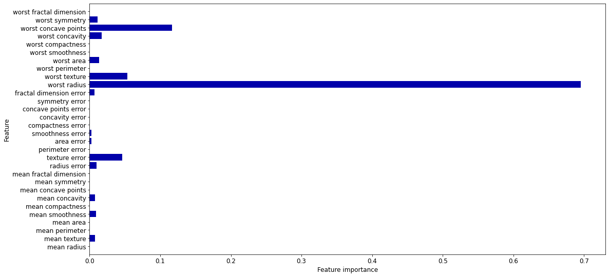
DecisionTreeClassifier also returns feature importances
tree.feature_importances_
In [0,1], sum up to 1
High values for features selected early (near the root)
# Feature importances sum up to 1
print("Feature importances:\n{}".format(tree.feature_importances_))
Feature importances:
[0.    0.008 0.    0.    0.009 0.    0.008 0.    0.    0.    0.01  0.046
 0.    0.002 0.002 0.    0.    0.    0.    0.007 0.695 0.054 0.    0.014
 0.    0.    0.017 0.117 0.011 0.   ]
def plot_feature_importances_cancer(model):
    n_features = cancer.data.shape[1]
    plt.barh(range(n_features), model.feature_importances_, align='center')
    plt.yticks(np.arange(n_features), cancer.feature_names)
    plt.xlabel("Feature importance")
    plt.ylabel("Feature")
    plt.ylim(-1, n_features)

plt.rcParams.update({'font.size': 8*fig_scale})
plt.rcParams["figure.figsize"] = (12*fig_scale,6*fig_scale)
plot_feature_importances_cancer(tree)
Decision tree regression#
Heuristic: Minimal quadratic distance
Consider splits at every data point for every variable (or halfway between)
Dividing the data on \(X_j\) at splitpoint \(s\) leads to the following half-spaces:
The best split, with predicted value \(c_i\) (mean of all values in the leaf) and actual value \(y_i\):
Assuming that the tree predicts \(y_i\) as the average of all \(x_i\) in the leaf:
with \(x_i\) being the i-th example in the data, with target value \(y_i\)
In scikit-learn#
Regression is done with DecisionTreeRegressor
def plot_decision_tree_regression(regr_1, regr_2):
    # Create a random dataset
    rng = np.random.RandomState(1)
    Xr = np.sort(5 * rng.rand(80, 1), axis=0)
    yr = np.sin(Xr).ravel()
    yr[::5] += 3 * (0.5 - rng.rand(16))

    # Fit regression model
    regr_1.fit(Xr, yr)
    regr_2.fit(Xr, yr)

    # Predict
    Xr_test = np.arange(0.0, 5.0, 0.01)[:, np.newaxis]
    y_1 = regr_1.predict(Xr_test)
    y_2 = regr_2.predict(Xr_test)

    # Plot the results
    plt.figure(figsize=(8,6))
    plt.scatter(Xr, yr, c="darkorange", label="data")
    plt.plot(Xr_test, y_1, color="cornflowerblue", label="max_depth=2", linewidth=2)
    plt.plot(Xr_test, y_2, color="yellowgreen", label="max_depth=5", linewidth=2)
    plt.xlabel("data")
    plt.ylabel("target")
    plt.title("Decision Tree Regression")
    plt.legend()
    plt.show()
from sklearn.tree import DecisionTreeRegressor
plt.rcParams["figure.figsize"] = (12*fig_scale,6*fig_scale)
regr_1 = DecisionTreeRegressor(max_depth=2)
regr_2 = DecisionTreeRegressor(max_depth=5)

plot_decision_tree_regression(regr_1,regr_2)
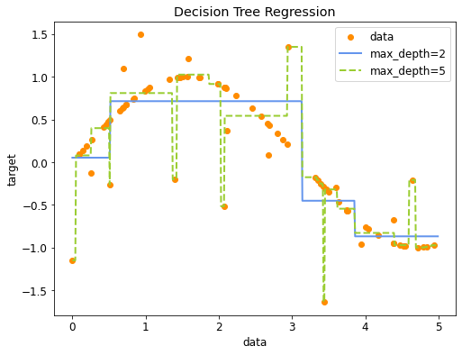
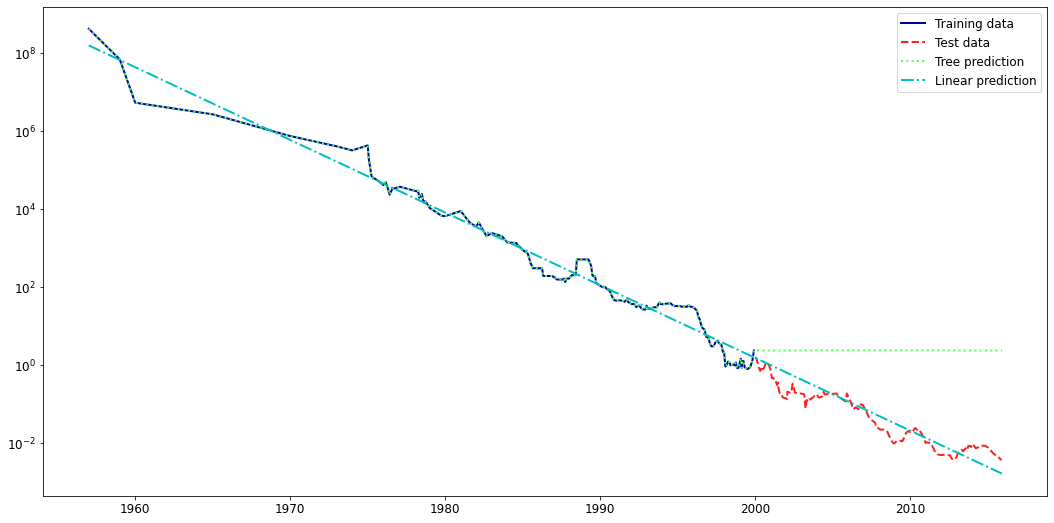
Note that decision trees do not extrapolate well.
The leafs return the same mean value no matter how far the new data point lies from the training examples.
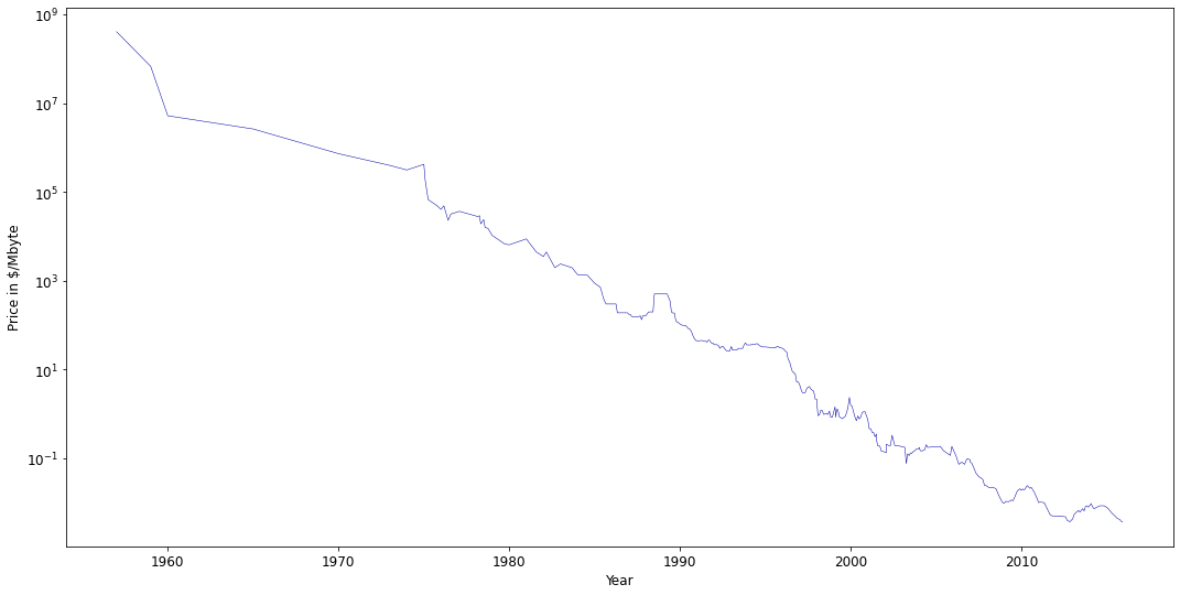
Example on the
ram_priceforecasting dataset
ram_prices = pd.read_csv('../data/ram_price.csv')

plt.semilogy(ram_prices.date, ram_prices.price)
plt.xlabel("Year")
plt.ylabel("Price in $/Mbyte");
from sklearn.tree import DecisionTreeRegressor
from sklearn.linear_model import LinearRegression

# Use historical data to forecast prices after the year 2000
data_train = ram_prices[ram_prices.date < 2000]
data_test = ram_prices[ram_prices.date >= 2000]

# predict prices based on date:
Xl_train = data_train.date[:, np.newaxis]
# we use a log-transform to get a simpler relationship of data to target
yl_train = np.log(data_train.price)

tree = DecisionTreeRegressor().fit(Xl_train, yl_train)
linear_reg = LinearRegression().fit(Xl_train, yl_train)

# predict on all data
X_all = ram_prices.date[:, np.newaxis]

pred_tree = tree.predict(X_all)
pred_lr = linear_reg.predict(X_all)

# undo log-transform
price_tree = np.exp(pred_tree)
price_lr = np.exp(pred_lr)
plt.rcParams['lines.linewidth'] = 2
plt.semilogy(data_train.date, data_train.price, label="Training data")
plt.semilogy(data_test.date, data_test.price, label="Test data")
plt.semilogy(ram_prices.date, price_tree, label="Tree prediction")
plt.semilogy(ram_prices.date, price_lr, label="Linear prediction")
plt.legend();
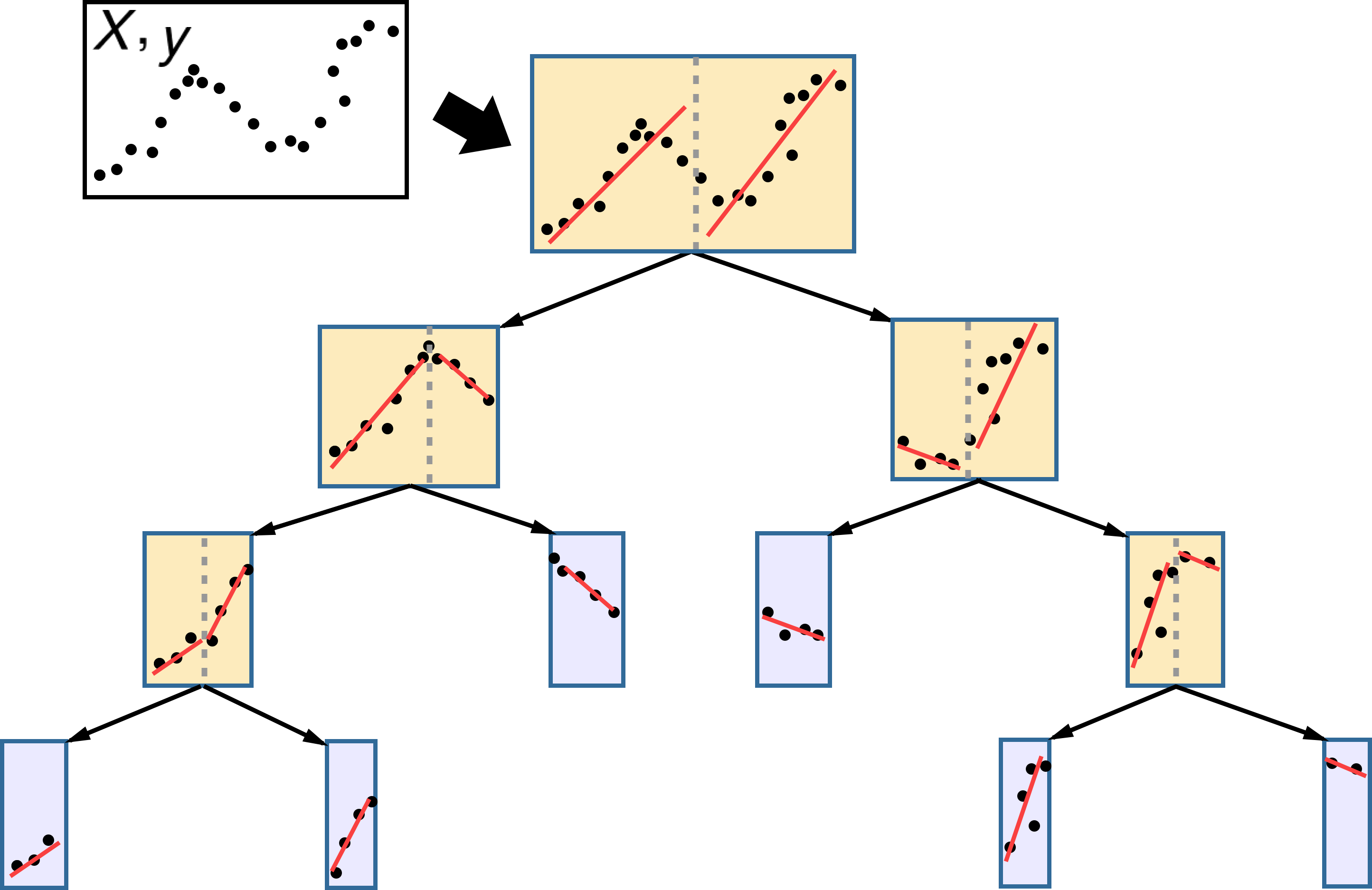
Model trees#
Instead of predicting a single value per leaf (e.g. mean value for regression), you can build a model on all the points remaining in a leaf
E.g. a linear regression model
Can learn more complex concepts, extrapolates better. Overfits easily.
Strengths, weaknesses and parameters#
Decision trees:
Work well with features on completely different scales, or a mix of binary and continuous features
Does not require normalization
Interpretable, easily visualized
Tend to overfit easily.
Pre-pruning: regularize by:
Setting a low
max_depth,max_leaf_nodesSetting a higher
min_samples_leaf(default=1)
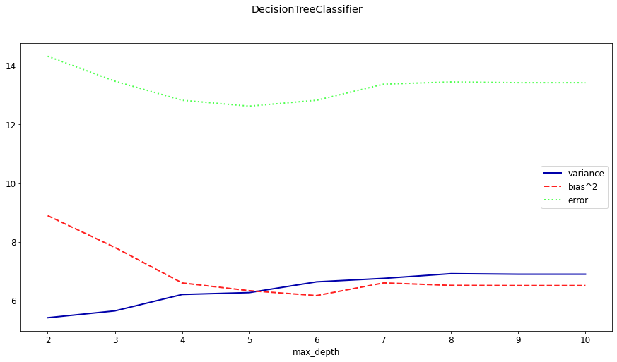
On under- and overfitting#
Let’s study which types of errors are made by decision trees
Deep trees have high variance but low bias
What if we built many deep trees and average them out to reduce variance?
Shallow trees have high bias but very low variance
What if we could correct the systematic mistakes to reduce bias?
from sklearn.model_selection import ShuffleSplit, train_test_split

# Bias-Variance Computation
def compute_bias_variance(clf, X, y):
    # Bootstraps
    n_repeat = 40 # 40 is on the low side to get a good estimate. 100 is better.
    shuffle_split = ShuffleSplit(test_size=0.33, n_splits=n_repeat, random_state=0)

    # Store sample predictions
    y_all_pred = [[] for _ in range(len(y))]

    # Train classifier on each bootstrap and score predictions
    for i, (train_index, test_index) in enumerate(shuffle_split.split(X)):
        # Train and predict
        clf.fit(X[train_index], y[train_index])
        y_pred = clf.predict(X[test_index])

        # Store predictions
        for j,index in enumerate(test_index):
            y_all_pred[index].append(y_pred[j])

    # Compute bias, variance, error
    bias_sq = sum([ (1 - x.count(y[i])/len(x))**2 * len(x)/n_repeat
                for i,x in enumerate(y_all_pred)])
    var = sum([((1 - ((x.count(0)/len(x))**2 + (x.count(1)/len(x))**2))/2) * len(x)/n_repeat
               for i,x in enumerate(y_all_pred)])
    error = sum([ (1 - x.count(y[i])/len(x)) * len(x)/n_repeat
            for i,x in enumerate(y_all_pred)])

    return np.sqrt(bias_sq), var, error

def plot_bias_variance(clf, X, y):
    bias_scores = []
    var_scores = []
    err_scores = []
    max_depth= range(2,11)

    for i in max_depth:
        b,v,e = compute_bias_variance(clf.set_params(random_state=0,max_depth=i),X,y)
        bias_scores.append(b)
        var_scores.append(v)
        err_scores.append(e)

    plt.figure(figsize=(10*fig_scale,5*fig_scale))
    plt.rcParams.update({'font.size': 12})
    plt.suptitle(clf.__class__.__name__)
    plt.plot(max_depth, var_scores,label ="variance" )
    plt.plot(max_depth, np.square(bias_scores),label ="bias^2")
    plt.plot(max_depth, err_scores,label ="error" )
    plt.xlabel("max_depth")
    plt.legend(loc="best")
    plt.show()

cancer = load_breast_cancer()
Xc, yc = cancer.data, cancer.target
dt = DecisionTreeClassifier()
plot_bias_variance(dt, Xc, yc)
Algorithm overview#
Name |
Representation |
Loss function |
Optimization |
Regularization |
|---|---|---|---|---|
Classification trees |
Decision tree |
Information Gain (KL div.) / Gini index |
Hunt’s algorithm |
Tree depth,… |
Regression trees |
Decision tree |
Min. quadratic distance |
Hunt’s algorithm |
Tree depth,… |
Model trees |
Decision tree + other models in leafs |
As above + used model’s loss |
Hunt’s algorithm + used model’s optimization |
Tree depth,… |