Lab 5: Bayesian models

We will first learn a GP regressor for an artificial, non-linear function to illustrate some basic aspects of GPs. To this end, we consider a sinusoidal function from which we sample a dataset.

# General imports
%matplotlib inline
import numpy as np
import pandas as pd
import matplotlib.pyplot as plt

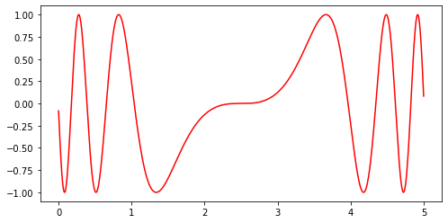
The function to predict and the dataset we create from it:

def f(x):
    """The function to predict."""
    return np.sin((x - 2.5) ** 3)

plt.figure(figsize=(8,4))
t = np.linspace(0,5,1000)
plt.plot(t, f(t), 'r', label = 'original f(x)')

[<matplotlib.lines.Line2D at 0x12d6a0580>]

The dataset we create based on the function:

# Dataset sampled from a sine function
rng = np.random.RandomState(4)
X_ = rng.uniform(0, 5, 1000)[:, np.newaxis]
y_ = f(X_).ravel()

def plot_gp(g, X_train, y_train, X_full, y_full, y_pred_mean, y_pred_std, use_title="yes"):
    """
    Visualizes the GP predictions, training points and original function
    
    Attributes:
    X_train -- The training data
    y_train -- The correct labels
    X_full -- The data to calculate predictions
    y_full -- The correct labels of the prediction data
    y_pred_mean -- the predicted means
    y_pred_std -- the predicted st. devs.
    """
    x_ = np.linspace(0, 5, 1000)[:,np.newaxis]
    
    idx = np.argsort(X_full[:,0])
    
    # Original function
    a = X_full[idx]
    b = y_full[idx]
    
    plt.figure(figsize=(8,4))
    plt.plot(a, 
             b, 'r', label = 'original f(x)')
    
    # Training points
    plt.scatter(X_train, y_train, c='r', s=50, zorder=10, edgecolors=(0, 0, 0))
    
    # Prediction 
    d = y_pred_mean[idx]
    e = y_pred_std[idx]
    plt.plot(a, d, 'k', lw=1, zorder=9)
    plt.fill_between(a[:,0], d - 1.96*e, d + 1.96*e, alpha=0.2, color='k')
    
    if use_title == "yes":
        plt.title("Posterior (kernel: %s)\n Log-Likelihood: %.3f"
              % (g.kernel_, g.log_marginal_likelihood(g.kernel_.theta)),
              fontsize=12)
    plt.tight_layout()

Exercise 1: visualizing predictions

Train a GP regressor with a RBF kernel with default hyperparameters on a 1% sample of the sine data. Note that by learning a GP the hyperparameters of the chosen kernel are tuned automatically. To visualize what the GP has learned, use the model to predict values for the entire dataset. Plot the original function, the predictions and the training data points. You can use the function plot_gp() to assist with plotting.

Exercise 2: reducing the uncertainty

Fit a model using 5% and 10% of the data. Now try setting n_restarts_optimizer in the GaussianProcessRegressor constructor. Plot the results. What differences do you see?

Exercise 3: Kernels

Like SVMs, kernels play a major role in GPs. Using a 5% sample of the data, train one GP with each of the following kernels:

• RBF

• RationalQuadratic

• ExpSineSquared

• DotProduct

• Matern

What differences do you see in the log-likelihood? Which model fit best the training data?

Exercise 4: Mauna Loa data

We now look at the problem of predicting the monthly average CO2 concentrations collected at the Mauna Loa Observatory in Hawaii, between 1958 and 2001. This is a time-series data.

from sklearn.datasets import fetch_openml

# originally from sci-kit learn
def load_mauna_loa_atmospheric_co2():
    ml_data = fetch_openml(data_id=41187, as_frame=False)
    months = []
    ppmv_sums = []
    counts = []

    y = ml_data.data[:, 0]
    m = ml_data.data[:, 1]
    month_float = y + (m - 1) / 12
    ppmvs = ml_data.target

    for month, ppmv in zip(month_float, ppmvs):
        if not months or month != months[-1]:
            months.append(month)
            ppmv_sums.append(ppmv)
            counts.append(1)
        else:
            # aggregate monthly sum to produce average
            ppmv_sums[-1] += ppmv
            counts[-1] += 1

    months = np.asarray(months).reshape(-1, 1)
    avg_ppmvs = np.asarray(ppmv_sums) / counts
    return months, avg_ppmvs


X_mauna, y_mauna = load_mauna_loa_atmospheric_co2()

Quick visualization:

#Quick visualization
plt.plot(X_mauna,y_mauna)
plt.xlabel('date')
plt.ylabel('co2')

Text(0, 0.5, 'co2')

Exercise 4.1

Signals like this usually consist of a combination of different “sub-signals”, e.g. a long-term component, a seasonal component, a noise component, and so on. When defining a GP kernel, you can combine multiple kernels, such as:

• A RBF kernel can be used to explain long-term, smooth patterns.

• The seasonal component can be modeled by an ExpSineSquared component.

• Small and medium-term irregularities can be modeled by a RationalQuadratic component.

• WhiteNoise kernel to model white noise.

Train a GP using the first 75% data points as training data using the kernel below. Experiment with removing one or more kernels and check the results visually (you can use plot_gp). What do you observe?

from sklearn.gaussian_process.kernels import WhiteKernel, RBF, ExpSineSquared, RationalQuadratic

k1 = 50.0**2 * RBF(length_scale=50.0)  # long term smooth rising trend
k2 = 2.0**2 * RBF(length_scale=100.0) \
    * ExpSineSquared(length_scale=1.0, periodicity=1.0,
                     periodicity_bounds="fixed")  # seasonal component
# medium term irregularities
k3 = 0.5**2 * RationalQuadratic(length_scale=1.0, alpha=1.0)
k4 = 0.1**2 * RBF(length_scale=0.1) \
    + WhiteKernel(noise_level=0.1**2,
                  noise_level_bounds=(1e-5, np.inf))  # noise terms

kernel = k1 + k2 +  k3 + k4