Lab 3: Ensembles

Using trees to detect trees

We will be using tree-based ensemble methods on the Covertype dataset. It contains about 100,000 observations of 7 types of trees (Spruce, Pine, Cottonwood, Aspen,…) described by 55 features describing elevation, distance to water, soil type, etc.

# Auto-setup when running on Google Colab
if 'google.colab' in str(get_ipython()):
    !pip install openml

# General imports
%matplotlib inline
import numpy as np
import pandas as pd
import matplotlib.pyplot as plt
import openml as oml
import seaborn as sns

# Download Covertype data. Takes a while the first time.
covertype = oml.datasets.get_dataset(180)
X, y, _, _ = covertype.get_data(target=covertype.default_target_attribute, dataset_format='array'); 
classes = covertype.retrieve_class_labels()
features = [f.name for i,f in covertype.features.items()][:-1]

classes

['Aspen',
 'Cottonwood_Willow',
 'Douglas_fir',
 'Krummholz',
 'Lodgepole_Pine',
 'Ponderosa_Pine',
 'Spruce_Fir']

features[0:20]

['elevation',
 'aspect',
 'slope',
 'horizontal_distance_to_hydrology',
 'Vertical_Distance_To_Hydrology',
 'Horizontal_Distance_To_Roadways',
 'Hillshade_9am',
 'Hillshade_Noon',
 'Hillshade_3pm',
 'Horizontal_Distance_To_Fire_Points',
 'wilderness_area1',
 'wilderness_area2',
 'wilderness_area3',
 'wilderness_area4',
 'soil_type_1',
 'soil_type_2',
 'soil_type_3',
 'soil_type_4',
 'soil_type_5',
 'soil_type_6']

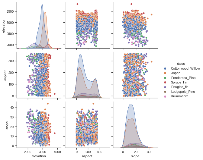
To understand the data a bit better, we can use a scatter matrix. From this, it looks like elevation is a relevant feature. Douglas Fir and Aspen grow at low elevations, while only Krummholz pines survive at very high elevations.

# Using seaborn to build the scatter matrix
# only first 3 columns, first 1000 examples
n_points = 1500
df = pd.DataFrame(X[:n_points,:3], columns=features[:3])
df['class'] = [classes[i] for i in y[:n_points]]
sns.set(style="ticks")
sns.pairplot(df, hue="class");

Exercise 1: Random Forests

Implement a function evaluate_RF that measures the performance of a Random Forest Classifier, using trees of (max) depth 2,8,32,64, for any number of trees in the ensemble (n_estimators). For the evaluation you should measure accuracy using 3-fold cross-validation. Use random_state=1 to ensure reproducibility. Finally, plot the results for at least 5 values of n_estimators ranging from 1 to 30. You can, of course, reuse code from earlier labs and assignments. Interpret the results. You can take a 50% subsample to speed the plotting.

Exercise 2: Other measures

Repeat the same plot but now use balanced_accuracy as the evaluation measure. See the documentation. Only use the optimal max_depth from the previous question. Do you see an important difference?

Exercise 3: Feature importance

Retrieve the feature importances according to the (tuned) random forest model. Which feature are most important?

Exercise 4: Feature selection

Re-build your tuned random forest, but this time only using the first 10 features. Return both the balanced accuracy and training time. Interpret the results.

Exercise 5: Confusion matrix

Do a standard stratified holdout and generate the confusion matrix of the tuned random forest. Which classes are still often confused?

Exercise 6: A second-level model

Build a binary model specifically to correctly choose between the first and the second class. Select only the data points with those classes and train a new random forest. Do a standard stratified split and plot the resulting ROC curve. Can we still improve the model by calibrating the threshold?

Exercise 7: Model calibration

For the trained binary random forest model, plot a calibration curve (see course notebook). Next, try to correct for this using Platt Scaling (or sigmoid scaling).

Probability calibration should be done on new data not used for model fitting. The class CalibratedClassifierCV uses a cross-validation generator and estimates for each split the model parameter on the train samples and the calibration of the test samples. The probabilities predicted for the folds are then averaged. Already fitted classifiers can be calibrated by CalibratedClassifierCV via the parameter cv=”prefit”. Read more

Exercise 8: Gradient Boosting

Implement a function evaluate_GB that measures the performance of GradientBoostingClassifier or the XGBoostClassifier for different learning rates (0.01, 0.1, 1, and 10). As before, use a 3-fold cross-validation. You can use a 5% stratified sample of the whole dataset. Finally plot the results for n_estimators ranging from 1 to 100. Run all the GBClassifiers with random_state=1 to ensure reproducibility.

Implement a function that plots the score of evaluate_GB for n_estimators = 10,20,30,…,100 on a linear scale.