Evaluation
- To know whether we can trust our method or system, we need to evaluate it.
- If you cannot measure it, you cannot improve it.
- Model selection: choose between different models in a data-driven way.
- Convince others that your work is meaningful
- Peers, leadership, clients, yourself(!)
- Keep evaluating relentlessly, adapt to changes
Designing Machine Learning systems
- Just running your favourite algorithm is usually not a great way to start
- Consider the problem at large
- Do you want to understand phenomena or do black box modelling?
- How to define and measure success? Are there costs involved?
- Do you have the right data? How can you make it better?
- Build prototypes early-on to evaluate the above.
- Analyze your model's mistakes
- Should you collect more, or additional data?
- Should the task be reformulated?
- Often a higher payoff than endless finetuning
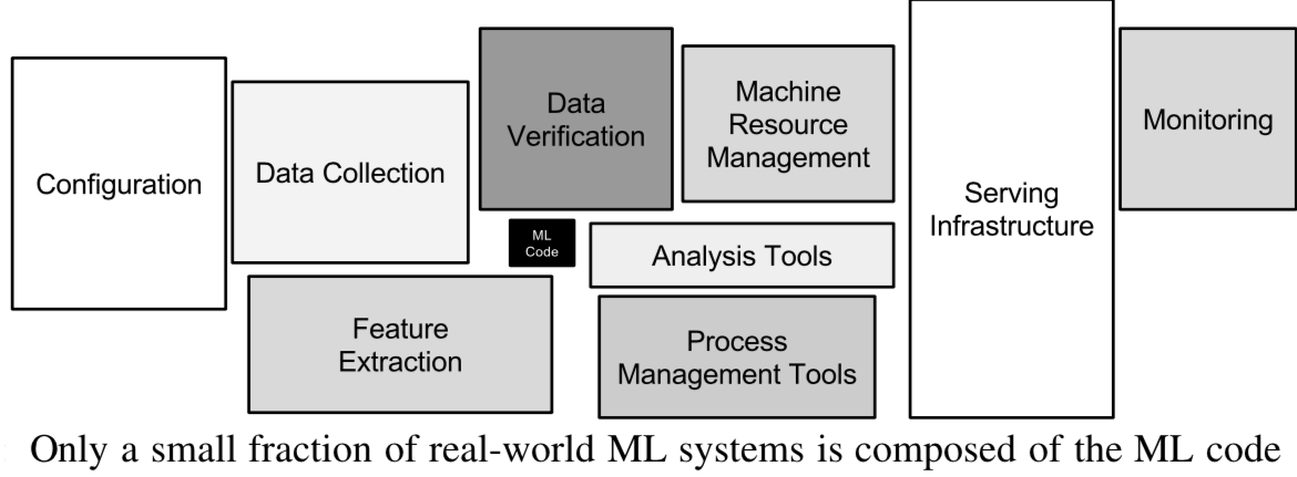
- Technical debt: creation-maintenance trade-off
- Very complex machine learning systems are hard/impossible to put into practice
- See 'Machine Learning: The High Interest Credit Card of Technical Debt'
Real world evaluations
- Evaluate predictions, but also how outcomes improve because of them
- Feedback loops: predictions are fed into the inputs, e.g. as new data, invalidating models
- Example: a medical recommendation model may change future measurements
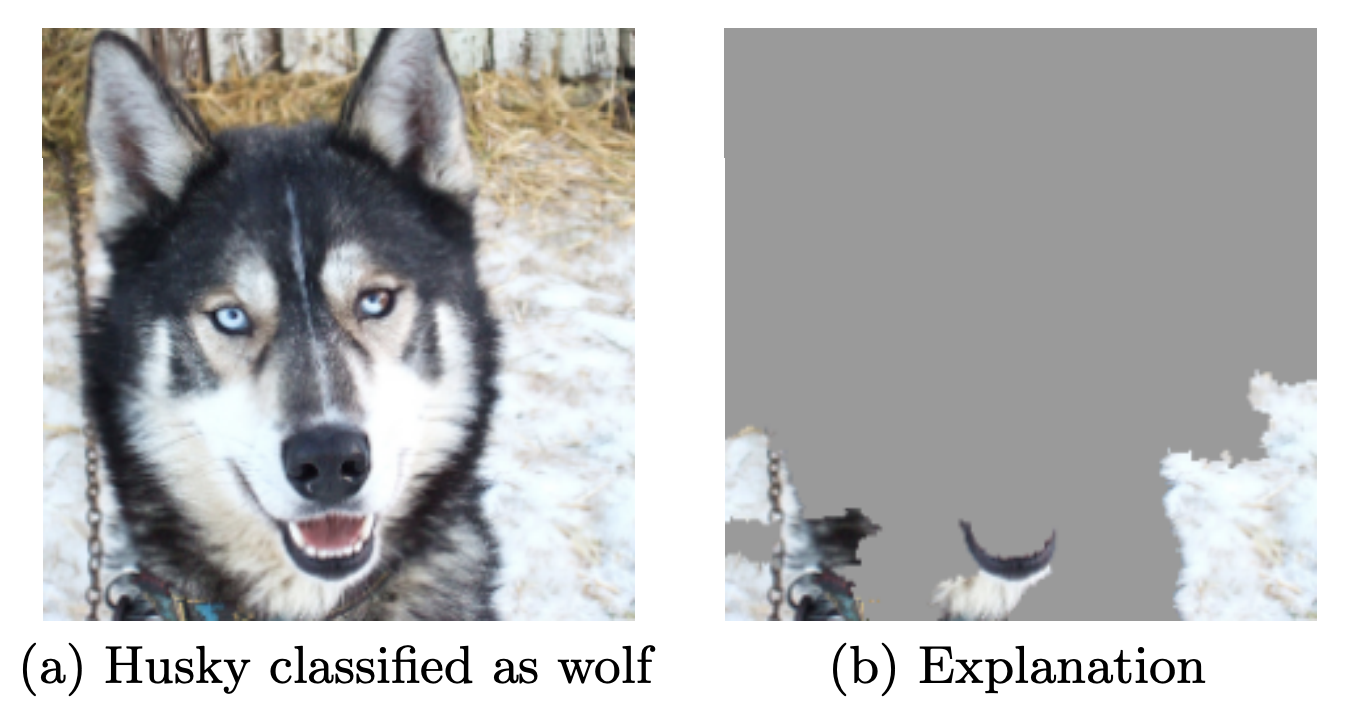
- The signal your model found may just be an artifact of your biased data
- When possible, try to interpret what your model has learned
- See 'Why Should I Trust You?' by Marco Ribeiro et al.
- Adversarial situations (e.g. spam filtering) can subvert your predictions
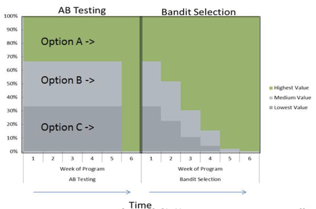
- Do A/B testing (or bandit testing) to evaluate algorithms in the wild
A/B and bandit testing
- Test a single innovation (or choose between two models)
- Have most users use the old system, divert small group to new system
- Evaluate and compare performance
- Bandit testing: smaller time intervals, direct more users to currently winning system
Performance estimation techniques
- We do not have access to future observations
- Always evaluate models as if they are predicting the future
- Set aside data for objective evaluation
- How?
The holdout (simple train-test split)
- Randomly split data (and corresponding labels) into training and test set (e.g. 75%-25%)
- Train (fit) a model on the training data, score on the test data
from sklearn.model_selection import (TimeSeriesSplit, KFold, ShuffleSplit, train_test_split,
                                     StratifiedKFold, GroupShuffleSplit,
                                     GroupKFold, StratifiedShuffleSplit)
from matplotlib.patches import Patch
np.random.seed(1338)
cmap_data = plt.cm.brg
cmap_group = plt.cm.Paired
cmap_cv = plt.cm.coolwarm
n_splits = 4

# Generate the class/group data
n_points = 100
X = np.random.randn(100, 10)

percentiles_classes = [.1, .3, .6]
y = np.hstack([[ii] * int(100 * perc)
               for ii, perc in enumerate(percentiles_classes)])

# Evenly spaced groups repeated once
rng = np.random.RandomState(42)
group_prior = rng.dirichlet([2]*10)
rng.multinomial(100, group_prior)
groups = np.repeat(np.arange(10), rng.multinomial(100, group_prior))
X_train, X_test, y_train, y_test = train_test_split(X, y, random_state=0)
fig = plt.figure()
ax = fig.add_subplot(111)
mglearn.discrete_scatter(X_train[:, 0], X_train[:, 1], y_train,
                         markers='o', ax=ax)
mglearn.discrete_scatter(X_test[:, 0], X_test[:, 1], y_test,
                         markers='^', ax=ax)
ax.legend(["Train class 0", "Train class 1", "Train class 2", "Test class 0",
                "Test class 1", "Test class 2"], ncol=6,  loc=(-0.1, 1.1));

K-fold Cross-validation
- Each random split can yield very different models (and scores)
- e.g. all easy (of hard) examples could end up in the test set
- Split data (randomly) into k equal-sized parts, called folds
- Create k splits, each time using a different fold as the test set
- Compute k evaluation scores, aggregate afterwards (e.g. take the mean)
- Examine the score variance to see how sensitive (unstable) models are
- Reduces sampling bias by testing on every point exactly once
- Large k gives better estimates (more training data), but is expensive
def plot_cv_indices(cv, X, y, group, ax, lw=2, show_groups=False, s=700, legend=True):
    """Create a sample plot for indices of a cross-validation object."""
    n_splits = cv.get_n_splits(X, y, group)

    # Generate the training/testing visualizations for each CV split
    for ii, (tr, tt) in enumerate(cv.split(X=X, y=y, groups=group)):
        # Fill in indices with the training/test groups
        indices = np.array([np.nan] * len(X))
        indices[tt] = 1
        indices[tr] = 0

        # Visualize the results
        ax.scatter([n_splits - ii - 1] * len(indices), range(len(indices)),
                   c=indices, marker='_', lw=lw, cmap=cmap_cv,
                   vmin=-.2, vmax=1.2, s=s)

    # Plot the data classes and groups at the end
    ax.scatter([-1] * len(X), range(len(X)),
               c=y, marker='_', lw=lw, cmap=cmap_data, s=s)
    yticklabels = ['class'] + list(range(1, n_splits + 1))

    if show_groups:
        ax.scatter([-2] * len(X), range(len(X)),
                   c=group, marker='_', lw=lw, cmap=cmap_group, s=s)
        yticklabels.insert(0, 'group')

    # Formatting
    ax.set(xticks=np.arange(-1 - show_groups, n_splits), xticklabels=yticklabels,
            ylabel='Sample index', xlabel="CV iteration",
            xlim=[-1.5 - show_groups, n_splits+.2], ylim=[-6, 100])
    ax.set_title('{}'.format(type(cv).__name__), fontsize=15)
    if legend:
        ax.legend([Patch(color=cmap_cv(.8)), Patch(color=cmap_cv(.2))],
                  ['Testing set', 'Training set'], loc=(1.02, .8))
    ax.spines['top'].set_visible(False)
    ax.spines['right'].set_visible(False)
    ax.spines['left'].set_visible(False)
    ax.spines['bottom'].set_visible(False)
    ax.set_yticks(())
    return ax
fig, ax = plt.subplots(figsize=(6, 3.5))
cv = KFold(5)
plot_cv_indices(cv, X, y, groups, ax, s=700);

Stratified K-Fold cross-validation
- If the data is unbalanced, some classes have many fewer samples
- Likely that some classes are not present in the test set
- Stratification: proportions between classes are conserved in each fold
- Order examples per class
- Separate the samples of each class in k sets (strata)
- Combine corresponding strate into folds
fig, ax = plt.subplots(figsize=(6, 3.9))
cv = StratifiedKFold(5)
plot_cv_indices(cv, X, y, groups, ax, s=700)
ax.set_ylim((-6, 100));

Can you explain this result?
kfold = KFold(n_splits=3)
print("Cross-validation scores KFold(n_splits=3):\n{}".format(
      cross_val_score(logreg, iris.data, iris.target, cv=kfold)))
from sklearn.model_selection import KFold, StratifiedKFold, cross_val_score
from sklearn.datasets import load_iris
from sklearn.linear_model import LogisticRegression

iris = load_iris()
logreg = LogisticRegression()
kfold = KFold(n_splits=3)
print("Cross-validation scores KFold(n_splits=3):\n{}".format(
      cross_val_score(logreg, iris.data, iris.target, cv=kfold)))
Leave-One-Out cross-validation
- k fold cross-validation with k equal to the number of samples
- Completely unbiased (in terms of data splits), but computationally expensive
- But: generalizes less well towards unseen data
- The training sets are correlated (overlap heavily)
- Overfits on the data used for (the entire) evaluation
- A different sample of the data can yield different results
- Recommended only for small datasets
Shuffle-Split cross-validation
- Additionally shuffles the data (only do this when the data is not ordered)
- Samples a number of samples (
train_size) randomly as the training set - Can also use a smaller (
test_size), handy when using very large datasets
fig, ax = plt.subplots(figsize=(6, 4))
cv = ShuffleSplit(8, test_size=.2)
plot_cv_indices(cv, X, y, groups, ax, n_splits, s=700)
ax.set_ylim((-6, 100))
ax.legend([Patch(color=cmap_cv(.8)), Patch(color=cmap_cv(.2))],
          ['Testing set', 'Training set'], loc=(.95, .8));

Note: this is related to bootstrapping:
- Sample n (total number of samples) data points, with replacement, as training set (the bootstrap)
- Use the unsampled (out-of-bootstrap) samples as the test set
- Repeat
n_itertimes, obtainingn_iterscores - Not supported in scikit-learn, only approximated
- Use Shuffle-Split with
train_size=0.66,test_size=0.34 - You can prove that bootstraps include 66% of all data points on average
- Use Shuffle-Split with
Repeated cross-validation
- Cross-validation is still biased in that the initial split can be made in many ways
- Repeated, or n-times-k-fold cross-validation:
- Shuffle data randomly, do k-fold cross-validation
- Repeat n times, yields n times k scores
- Unbiased, very robust, but n times more expensive
from sklearn.model_selection import RepeatedStratifiedKFold
from matplotlib.patches import Rectangle
fig, ax = plt.subplots(figsize=(10, 3.9))
cv = RepeatedStratifiedKFold(n_splits=5, n_repeats=3)
plot_cv_indices(cv, X, y, groups, ax, lw=2, s=400, legend=False)
ax.set_ylim((-6, 102))
xticklabels = ["class"] + [f"{repeat}x{split}" for repeat in range(1, 4) for split in range(1, 6)]
ax.set_xticklabels(xticklabels)
for i in range(3):
    rect = Rectangle((-.5 + i * 5, -2.), 5, 103, edgecolor='k', facecolor='none')
    ax.add_artist(rect)

Cross-validation with groups
- Sometimes the data contains inherent groups:
- Multiple samples from same patient, images from same person,...
- With normal cross-validation, data from the same person may end up in the training and test set
- We want to measure how well the model generalizes to other people
- Make sure that data from one person are in either the train or test set
- This is called grouping or blocking
- Leave-one-subject-out cross-validation: test set for each subject
fig, ax = plt.subplots(figsize=(6, 3.9))
cv = GroupKFold(5)
plot_cv_indices(cv, X, y, groups, ax, s=700, show_groups=True)
ax.set_ylim((-6, 100));

Time series
When the data is ordered, random test sets are not a good idea
import pandas as pd
approval = pd.read_csv("https://projects.fivethirtyeight.com/trump-approval-data/approval_topline.csv")
adults = approval.groupby("subgroup").get_group('Adults')
adults = adults.set_index('modeldate')[::-1]
adults.approve_estimate.plot()
ax = plt.gca()
plt.rcParams["figure.figsize"] = [8,4]
ax.set_xlabel("")
xlim, ylim = ax.get_xlim(), ax.get_ylim()
for i in range(20):
    rect = Rectangle((np.random.randint(0, xlim[1]), ylim[0]), 10, ylim[1]-ylim[0], facecolor='#FFAAAA')
    ax.add_artist(rect)
plt.title("Presidential approval estimates by fivethirtyeight")
plt.legend([rect], ['Random Test Set'] );

Time series
- Test-then-train (prequential evaluation)
- Every new sample is evaluated on once, then added to the training set
- Can also be done in batches (of n samples at a time)
TimeSeriesSplit- In the kth split, the first k folds are used as the train set and the (k+1)th fold as the test set
- Can also be done with a maximum training set size: more robust against concept drift
from sklearn.utils import shuffle
fig, ax = plt.subplots(figsize=(6, 3.9))
cv = TimeSeriesSplit(5, max_train_size=20)
plot_cv_indices(cv, X, shuffle(y), groups, ax, s=700, lw=2)
ax.set_ylim((-6, 100))
ax.set_title("TimeSeriesSplit(5, max_train_size=20)");

Choosing a performance estimation procedure
No strict rules, only guidelines:
- Always use stratification for classification (sklearn does this by default)
- Use holdout for very large datasets (e.g. >1.000.000 examples)
- Or when learners don't always converge (e.g. deep learning)
- Choose k depending on dataset size and resources
- Use leave-one-out for small datasets (e.g. <500 examples)
- Use cross-validation otherwise
- Most popular (and theoretically sound): 10-fold CV
- Literature suggests 5x2-fold CV is better
- Use grouping or leave-one-subject-out for grouped data
- Use train-then-test for time series
Evaluation Metrics and scoring
Keep the end-goal in mind
Evaluation vs Optimization
- Each algorithm optimizes a given objective function (on the training data)
- E.g. remember L2 loss in Ridge regression $$\mathcal{L}_{ridge} = \sum_{i}(y_i - \sum_{j} x_{i,j}w_j)^2 + \alpha \sum_{i} w_i^2$$
- The choice of function is limited by what can be efficiently optimized
- E.g. gradient descent requires a differentiable loss function
- However, we evaluate the resulting model with a score that makes sense in the real world
- E.g. percentage of correct predictions (on a test set)
- We also tune the algorithm's hyperparameters to maximize that score
Binary classification
- We have a positive and a negative class
- 2 different kind of errors:
- False Positive (type I error): model predicts positive while the true label is negative
- False Negative (type II error): model predicts negative while the true label is positive
- They are not always equally important
- Which side do you want to err on for a medical test?
Confusion matrices
- We can represent all predictions (correct and incorrect) in a confusion matrix
- n by n array (n is the number of classes)
- Rows correspond to true classes, columns to predicted classes
- Each entry counts how often a sample that belongs to the class corresponding to the row was classified as the class corresponding to the column.
- For binary classification, we label these true negative (TN), true positive (TP), false negative (FN), false positive (FP)
mglearn.plots.plot_binary_confusion_matrix()

Predictive accuracy
- Accuracy is one of the measures we can compute based on the confusion matrix:
- In sklearn: use
confusion_matrixandaccuracy_scorefromsklearn.metrics. - Accuracy is also the default evaluation measure for classification
from sklearn.metrics import accuracy_score, confusion_matrix
from sklearn.model_selection import train_test_split
from sklearn.datasets import load_breast_cancer
from sklearn.linear_model import LogisticRegression
data = load_breast_cancer()
X_train, X_test, y_train, y_test = train_test_split(
    data.data, data.target, stratify=data.target, random_state=0)
lr = LogisticRegression().fit(X_train, y_train)
y_pred = lr.predict(X_test)

print("confusion_matrix(y_test, y_pred): \n", confusion_matrix(y_test, y_pred))
print("accuracy_score(y_test, y_pred): ", accuracy_score(y_test, y_pred))
print("model.score(X_test, y_test): ", lr.score(X_test, y_test))
The problem with accuracy: imbalanced datasets
- The type of error plays an even larger role if the dataset is imbalanced
- One class is much more frequent than the other, e.g. credit fraud
- Is a 99.99% accuracy good enough?
- Are these three models really equally good?
plot_measure(accuracy_score)

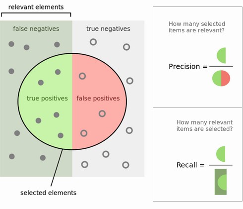
Precision is used when the goal is to limit FPs
- Clinical trails: you only want to test drugs that really work
- Search engines: you want to avoid bad search results
from sklearn.metrics import precision_score
plot_measure(precision_score)

Recall is used when the goal is to limit FNs
- Cancer diagnosis: you don't want to miss a serious disease
- Search engines: You don't want to omit important hits
- Also know as sensitivity, hit rate, true positive rate (TPR)
from sklearn.metrics import recall_score
plot_measure(recall_score)

Comparison
F1-score or F1-measure trades off precision and recall:
\begin{equation} \text{F1} = 2 \cdot \frac{\text{precision} \cdot \text{recall}}{\text{precision} + \text{recall}} \end{equation}from sklearn.metrics import f1_score
plot_measure(f1_score)

Classification measure Zoo
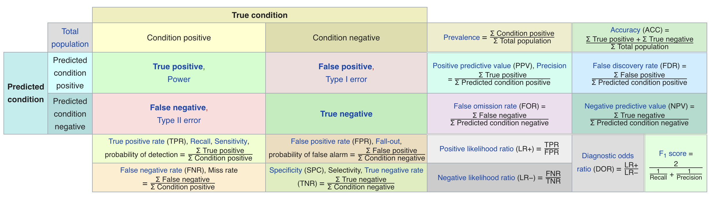 https://en.wikipedia.org/wiki/Precision_and_recall
Averaging scores per class
- Study the scores by class (in scikit-learn:
classification_report)- One class viewed as positive, other(s) als negative
- Support: number of samples in each class
- Last line: weighted average over the classes (weighted by number of samples in each class)
- Averaging for scoring measure R across C classes (also for multiclass):
- micro: count total number of TP, FP, TN, FN
- macro $$\frac{1}{C} \sum_{c \in C} R(y_c,\hat{y_c})$$
- weighted ($w_c$: ratio of examples of class $c$) $$\sum_{c \in C} w_c R(y_c,\hat{y_c})$$
from sklearn.metrics import classification_report

def report(y_pred):
    print(classification_report(y_true, y_pred))
    fig, ax = plt.subplots(figsize=(2, 2))
    plt.rcParams['figure.dpi'] = 100 # Use 300 for PDF, 100 for slides
    plot_confusion_matrix(confusion_matrix(y_true, y_pred), cmap='gray_r', ax=ax,
                          xticklabels=["N", "P"], yticklabels=["N", "P"], xtickrotation=0, vmin=0, vmax=100)
    plt.tight_layout();
report(y_pred_1)

report(y_pred_2)

report(y_pred_3)

Uncertainty estimates from classifiers
- Classifiers can often provide uncertainty estimates of predictions.
- Remember that linear models actually return a numeric value.
- When $\hat{y}<0$, predict class -1, otherwise predict class +1 $$\hat{y} = w_0 * x_0 + w_1 * x_1 + ... + w_p * x_p + b $$
- In practice, you are often interested in how certain a classifier is about each class prediction (e.g. cancer treatments).
Scikit-learn offers 2 functions. Often, both are available for every learner, but not always.
- decision_function: returns floating point value for each sample
- predict_proba: return probability for each class
The Decision Function
In the binary classification case, the return value of decision_function encodes how strongly the model believes a data point to belong to the “positive” class.
- Positive values indicate a preference for the "positive" class
- Negative values indicate a preference for the "negative" (other) class
# create and split a synthetic dataset
from sklearn.linear_model import LogisticRegression
from sklearn.datasets import make_blobs
X, y = make_blobs(centers=2, cluster_std=2.5, random_state=8)

# we rename the classes "blue" and "red"
y_named = np.array(["blue", "red"])[y]

# we can call train test split with arbitrary many arrays
# all will be split in a consistent manner
X_train, X_test, y_train_named, y_test_named, y_train, y_test = \
    train_test_split(X, y_named, y, random_state=0)

# build the logistic regression model
lr = LogisticRegression()
lr.fit(X_train, y_train_named)

# get the decision function
dec = lr.decision_function(X_test)

mglearn.plots.plot_2d_separator(lr, X)
mglearn.discrete_scatter(X[:, 0], X[:, 1], y);
plt.rcParams['figure.dpi'] = 90

for i, v in enumerate(dec):
    plt.annotate("{:.2f}".format(v), (X_test[i,0],X_test[i,1]),
                 textcoords="offset points", xytext=(0,7))

- The range of decision_function can be arbitrary, and depends on the data and the model parameters. This makes it sometimes hard to interpret.
- We can visualize the decision function as follows, with the actual decision boundary left and the values of the decision boudaries color-coded on the right.
- Note how the test examples are labeled depending on the decision function.
fig, axes = plt.subplots(1, 2, figsize=(13, 5))

mglearn.tools.plot_2d_separator(lr, X, ax=axes[0], alpha=.4,
                                fill=True, cm=mglearn.cm2)
scores_image = mglearn.tools.plot_2d_scores(lr, X, ax=axes[1],
                                            alpha=.4, cm=mglearn.ReBl)

for ax in axes:
    # plot training and test points
    mglearn.discrete_scatter(X_test[:, 0], X_test[:, 1], y_test,
                             markers='^', ax=ax)
    mglearn.discrete_scatter(X_train[:, 0], X_train[:, 1], y_train,
                             markers='o', ax=ax)
    ax.set_xlabel("Feature 0")
    ax.set_ylabel("Feature 1")
cbar = plt.colorbar(scores_image, ax=axes.tolist())
cbar.set_alpha(1)
cbar.draw_all()
axes[0].legend(["Test class 0", "Test class 1", "Train class 0",
                "Train class 1"], ncol=4, loc=(.1, 1.1));

Predicting probabilities
The output of predict_proba is a probability for each class, with one column per class. They sum up to 1.
print("Shape of probabilities: {}".format(lr.predict_proba(X_test).shape))
# show the first few entries of predict_proba
print("Predicted probabilities:\n{}".format(
      lr.predict_proba(X_test[:6])))
We can visualize them again. Note that the gradient looks different now.
fig, axes = plt.subplots(1, 2, figsize=(13, 5))

mglearn.tools.plot_2d_separator(
    lr, X, ax=axes[0], alpha=.4, fill=True, cm=mglearn.cm2)
scores_image = mglearn.tools.plot_2d_scores(
    lr, X, ax=axes[1], alpha=.5, cm=mglearn.ReBl, function='predict_proba')

for ax in axes:
    # plot training and test points
    mglearn.discrete_scatter(X_test[:, 0], X_test[:, 1], y_test,
                             markers='^', ax=ax)
    mglearn.discrete_scatter(X_train[:, 0], X_train[:, 1], y_train,
                             markers='o', ax=ax)
    ax.set_xlabel("Feature 0")
    ax.set_ylabel("Feature 1")
# don't want a transparent colorbar
cbar = plt.colorbar(scores_image, ax=axes.tolist())
cbar.set_alpha(1)
cbar.draw_all()
axes[0].legend(["Test class 0", "Test class 1", "Train class 0",
                "Train class 1"], ncol=4, loc=(.1, 1.1));

Interpreting probabilities
- The class with the highest probability is predicted.
- How well the uncertainty actually reflects uncertainty in the data depends on the model and the parameters.
- An overfitted model tends to make more certain predictions, even if they might be wrong.
- A model with less complexity usually has more uncertainty in its predictions.
- A model is called calibrated if the reported uncertainty actually matches how correct it is
— A prediction made with 70% certainty would be correct 70% of the time.
- LogisticRegression returns well calibrated predictions by default as it directly optimizes log-loss
- Linear SVM are not well calibrated. They are biased towards points close to the decision boundary.
- Calibration techniques can calibrate models in post-processing.
Model calibration
from sklearn.svm import LinearSVC, SVC
from sklearn.tree import DecisionTreeClassifier
from sklearn.ensemble import RandomForestClassifier
from sklearn.calibration import calibration_curve

from sklearn.datasets import fetch_covtype
from sklearn.utils import check_array

def load_data(dtype=np.float32, order='C', random_state=13):
    ######################################################################
    # Load covertype dataset (downloads it from the web, might take a bit)
    # TODO: Use OpenML version
    data = fetch_covtype(download_if_missing=True, shuffle=True,
                         random_state=random_state)
    X = check_array(data['data'], dtype=dtype, order=order)
    # make it bineary classification
    y = (data['target'] != 1).astype(np.int)

    # Create train-test split (as [Joachims, 2006])
    n_train = 522911
    X_train = X[:n_train]
    y_train = y[:n_train]
    X_test = X[n_train:]
    y_test = y[n_train:]

    # Standardize first 10 features (the numerical ones)
    mean = X_train.mean(axis=0)
    std = X_train.std(axis=0)
    mean[10:] = 0.0
    std[10:] = 1.0
    X_train = (X_train - mean) / std
    X_test = (X_test - mean) / std
    return X_train, X_test, y_train, y_test

X_train, X_test, y_train, y_test = load_data()

# subsample training set by a factor of 10:
X_train = X_train[::10]
y_train = y_train[::10]

#probs = lr.predict_proba(X_test)[:, 1]
#prob_true, prob_pred = calibration_curve(y_test, probs, n_bins=5)

from sklearn.linear_model import LogisticRegressionCV
lr = LogisticRegressionCV().fit(X_train, y_train)

def plot_calibration_curve(y_true, y_prob, n_bins=5, ax=None, hist=True, normalize=False):
    prob_true, prob_pred = calibration_curve(y_true, y_prob, n_bins=n_bins, normalize=normalize)
    if ax is None:
        ax = plt.gca()
    if hist:
        ax.hist(y_prob, weights=np.ones_like(y_prob) / len(y_prob), alpha=.4,
               bins=np.maximum(10, n_bins))
    ax.plot([0, 1], [0, 1], ':', c='k')
    curve = ax.plot(prob_pred, prob_true, marker="o")

    ax.set_xlabel("predicted probability")
    ax.set_ylabel("fraction of positive samples")

    ax.set(aspect='equal')
    return curve

fig, axes = plt.subplots(1, 3, figsize=(8, 8))
for ax, clf in zip(axes, [LogisticRegressionCV(), DecisionTreeClassifier(),
                          RandomForestClassifier()]):
        # use predict_proba is the estimator has it
        scores = clf.fit(X_train, y_train).predict_proba(X_test)[:, 1]
        plot_calibration_curve(y_test, scores, n_bins=20, ax=ax)
        ax.set_title(clf.__class__.__name__)

plt.tight_layout();

Model calibration
- Build another model, mapping classifier probabilities to better probabilities!
1d model! (or more for multi-class) $$f_{calib}(s(x))≈p(y)$$
s(x) is score given by model, usually
- Can also work with models that don’t even provide probabilities! Need model for f_{calib}, need to decide what data to train it on.
- Can train on training set, causes overfit
- Can train using cross-validation, slower
Platt Scaling
Use a logistic sigmoid for $f_{calib}$ $$f_{platt}=\frac{1}{1+\exp(−ws(x)−b)}$$
Basically learning a 1d logistic regression (+ some tricks)
- Works well for SVMs
Isotonic regression
- Very flexible way to specify $f_{calib}
- Learns arbitrary monotonically increasing step-functions in 1d.
- Groups data into constant parts, steps in between.
- Optimum monotone function on training data (wrt MSE)

Taking uncertainty into account
- Remember that many classifiers actually return a probability per class
- We can retrieve it with
decision_functionandpredict_proba
- We can retrieve it with
- For binary classification, we threshold at 0 for
decision_functionand 0.5 forpredict_probaby default - However, depending on the evaluation measure, you may want to threshold differently to fit your goals
- For instance, when a FP is much worse than a FN
- This is called threshold calibration
- Imagine that we want to avoid misclassifying a positive (red) point
- Points within decision boundary (black line) are classified positive
- Lowering the decision treshold (bottom figure): fewer FN, more FP
plt.rcParams['figure.dpi'] = 80
mglearn.plots.plot_decision_threshold()

- Studying the classification report, we see that lowering the threshold yields:
- higher recall for class 1 (we risk more FPs in exchange for more TP)
- lower precision for class 1
- We can often trade off precision for recall
plt.rcParams['figure.dpi'] = 100
print("Threshold 0")
print(classification_report(y_test, svc.predict(X_test)))
print("Threshold -0.8")
y_pred_lower_threshold = svc.decision_function(X_test) > -.8
print(classification_report(y_test, y_pred_lower_threshold))
Precision-Recall curves
- As we've seen, you can trade off precision for recall by changing the decision threshold
- The best trade-off depends on your application, driven by real-world goals.
- You can have arbitrary high recall, but you often want reasonable precision, too.
- Plotting precision against recall for all possible thresholds yields a precision-recall curve
- It helps answer multiple questions:
- Threshold calibration: what's the best achievable precision-recall tradeoff?
- How much more precision can I gain without losing too much recall?
- Which models offer the best trade-offs?
from sklearn.metrics import precision_recall_curve
precision, recall, thresholds = precision_recall_curve(
    y_test, svc.decision_function(X_test))
- The default threshold (threshold zero) gives a certain precision and recall
- Lower the threshold to gain higher recall (move right)
- Increase the threshold to gain higher precision (move left)
- The curve is often jagged: increasing the threshold leaves fewer and fewer positive predictions, so precision ($\frac{TP}{TP+FP}$) can change dramatically
- The closer the curve stays to the upper-right corner, the better
- Here, it is possible to still get a precision of 0.55 with recall 0.9
# create a similar dataset as before, but with more samples
# to get a smoother curve
X, y = make_blobs(n_samples=(4000, 500), centers=2, cluster_std=[7.0, 2],
                  random_state=22)
X_train, X_test, y_train, y_test = train_test_split(X, y, random_state=0)

svc = SVC(gamma=.05).fit(X_train, y_train)

precision, recall, thresholds = precision_recall_curve(
    y_test, svc.decision_function(X_test))
# find threshold closest to zero:
close_zero = np.argmin(np.abs(thresholds))
plt.plot(recall[close_zero], precision[close_zero], 'o', markersize=10,
         label="threshold zero", fillstyle="none", c='k', mew=2)

plt.plot(recall, precision, label="precision recall curve")
plt.ylabel("Precision")
plt.xlabel("Recall")
plt.legend(loc="best");

Model selection
- Different classifiers offer different trade-offs
- RandomForest (in red) performs better at the extremes, SVM better in center
- In applications we may only care about a specific region (e.g. very high recall)
from sklearn.ensemble import RandomForestClassifier

rf = RandomForestClassifier(n_estimators=100, random_state=0, max_features=2)
rf.fit(X_train, y_train)

# RandomForestClassifier has predict_proba, but not decision_function
# Only pass probabilities for the positive class
precision_rf, recall_rf, thresholds_rf = precision_recall_curve(
    y_test, rf.predict_proba(X_test)[:, 1])

plt.plot(recall, precision, label="svc")

plt.plot(recall[close_zero], precision[close_zero], 'o', markersize=10,
         label="threshold zero svc", fillstyle="none", c='k', mew=2)

plt.plot(recall_rf, precision_rf, label="rf")

close_default_rf = np.argmin(np.abs(thresholds_rf - 0.5))
plt.plot( recall_rf[close_default_rf], precision_rf[close_default_rf], '^', c='k',
         markersize=10, label="threshold 0.5 rf", fillstyle="none", mew=2)
plt.ylabel("Precision")
plt.xlabel("Recall")
plt.legend(loc="best");

AUPRC
- The area under the precision-recall curve (AUPRC) is often used as a general evaluation measure
- This is a good general measure, but also hides the subtleties we saw in the curve
from sklearn.metrics import average_precision_score
ap_rf = average_precision_score(y_test, rf.predict_proba(X_test)[:, 1])
ap_svc = average_precision_score(y_test, svc.decision_function(X_test))
print("Average precision of random forest: {:.3f}".format(ap_rf))
print("Average precision of svc: {:.3f}".format(ap_svc))
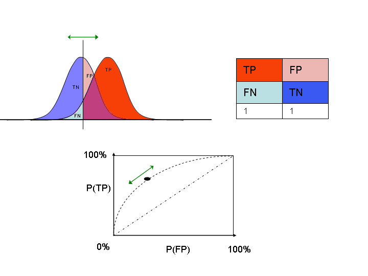
Receiver Operating Characteristics (ROC)
- We can also trade off recall (or true positive rate) $\textit{TPR}= \frac{TP}{TP + FN}$ with false positive rate $\textit{FPR} = \frac{FP}{FP + TN}$
- Varying the decision threshold yields the ROC curve
- Lower the threshold to gain more recall (move right)
- Increase the threshold to reduce FPs (move left)
plt.rcParams['savefig.dpi'] = 100 # Use 300 for PDF, 100 for slides
from sklearn.metrics import roc_curve
fpr, tpr, thresholds = roc_curve(y_test, svc.decision_function(X_test))

plt.plot(fpr, tpr, label="ROC Curve")
plt.xlabel("FPR")
plt.ylabel("TPR (recall)")
# find threshold closest to zero:
close_zero = np.argmin(np.abs(thresholds))
plt.plot(fpr[close_zero], tpr[close_zero], 'o', markersize=10,
         label="threshold zero", fillstyle="none", c='k', mew=2)
plt.legend(loc=4);

Visualization
- Horizontal axis represents the decision function. Every predicted point is on it.
- The blue probability density shows the actual negative points. The red one is for the positive points.
- Vertical line is the decision threshold: every point to the left is predicted negative (TN or FN) and vice versa (TP or FP).
- Increase threshold: fewer FP and TP: point on ROC curve moves leftward
Model selection
- Again, we can compare multiple models by looking at the ROC curves
- We can calibrate the threshold depending on whether we need high recall or low FPR
- We can select between algorithms (or hyperparameters) depending on the involved costs
from sklearn.metrics import roc_curve
fpr_rf, tpr_rf, thresholds_rf = roc_curve(y_test, rf.predict_proba(X_test)[:, 1])

plt.plot(fpr, tpr, label="ROC Curve SVC")
plt.plot(fpr_rf, tpr_rf, label="ROC Curve RF")

plt.xlabel("FPR")
plt.ylabel("TPR (recall)")
plt.plot(fpr[close_zero], tpr[close_zero], 'o', markersize=10,
         label="threshold zero SVC", fillstyle="none", c='k', mew=2)
close_default_rf = np.argmin(np.abs(thresholds_rf - 0.5))
plt.plot(fpr_rf[close_default_rf], tpr_rf[close_default_rf], '^', markersize=10,
         label="threshold 0.5 RF", fillstyle="none", c='k', mew=2)

plt.legend(loc=4);

Calculating costs
- A certain amount of FP and FN can be translated to a cost: $$\text{total cost} = \text{FPR} * cost_{FP} + (1-\text{TPR}) * cost_{FN}$$
- This yields different isometrics (lines of equal cost) in ROC space
- The optimal threshold is the point on the ROC curve where the cost is minimal
import ipywidgets as widgets
from ipywidgets import interact, interact_manual

# Cost function
def cost(fpr, tpr, cost_FN, cost_FP):
    return fpr * cost_FP + (1 - tpr) * cost_FN;

@interact
def plot_isometrics(c_FN=(1,10.0,1.0), c_FP=(1,10.0,1.0)):
    plt.rcParams['savefig.dpi'] = 100 # Use 300 for PDF, 100 for slides
    from sklearn.metrics import roc_curve
    fpr, tpr, thresholds = roc_curve(y_test, svc.decision_function(X_test))

    # get minimum
    costs = [cost(fpr[x],tpr[x],c_FN,c_FP) for x in range(len(thresholds))]
    min_cost = np.min(costs)
    min_thres = np.argmin(costs)

    # plot contours
    x = np.arange(0.0, 1.1, 0.1)
    y = np.arange(0.0, 1.1, 0.1)
    Xp, Yp = np.meshgrid(x, y)
    costs = [cost(f, t, c_FN, c_FP) for f, t in zip(Xp,Yp)]

    plt.plot(fpr, tpr, label="ROC Curve")
    levels = np.linspace(np.array(costs).min(), np.array(costs).max(), 10)
    levels = np.sort(np.append(levels, min_cost))
    CS = plt.contour(Xp, Yp, costs, levels)
    plt.clabel(CS, inline=1, fontsize=10)

    plt.xlabel("FPR")
    plt.ylabel("TPR (recall)")
    # find threshold closest to zero:
    plt.plot(fpr[min_thres], tpr[min_thres], 'o', markersize=4,
             label="optimal", fillstyle="none", c='k', mew=2)
    plt.legend(loc=4);
    plt.title("Isometrics, cost_FN: {}, cost_FP: {}".format(c_FN, c_FP))
    plt.show()
for cFP in [1, 10]:
    plot_isometrics(1,cFP)


Area under the ROC curve
- A useful summary measure is the area under the ROC curve (AUROC or AUC)
- Key benefit: 'sensitive' to class imbalance
- Random guessing always yields TPR=FPR
- All points are on the diagonal line, hence an AUC of 0.5
from sklearn.metrics import roc_auc_score
from sklearn.dummy import DummyClassifier
rf_auc = roc_auc_score(y_test, rf.predict_proba(X_test)[:, 1])
svc_auc = roc_auc_score(y_test, svc.decision_function(X_test))
dummy = DummyClassifier().fit(X_train, y_train)
dummy_auc = roc_auc_score(y_test, dummy.predict_proba(X_test)[:, 1])
print("AUC for Random Forest: {:.3f}".format(rf_auc))
print("AUC for SVC: {:.3f}".format(svc_auc))
print("AUC for dummy classifier: {:.3f}".format(dummy_auc))
Example: unbalanced dataset (10% positive, 90% negative):
- 3 models: overfitting ($\gamma=1.0$), good ($\gamma=0.01$), underfitting ($\gamma$=1e-5)
- ACC is the same (we might be random guessing), AUC is more informative
from sklearn.datasets import load_digits

digits = load_digits()
y = digits.target == 9

X_train, X_test, y_train, y_test = train_test_split(
    digits.data, y, random_state=0)

plt.figure()

for gamma in [1, 0.01, 0.00001]:
    svc = SVC(gamma=gamma).fit(X_train, y_train)
    accuracy = svc.score(X_test, y_test)
    auc = roc_auc_score(y_test, svc.decision_function(X_test))
    fpr, tpr, _ = roc_curve(y_test , svc.decision_function(X_test))
    print("gamma = {:.1e}  ACC = {:.2f}  AUC = {:.4f}".format(
            gamma, accuracy, auc))
    plt.plot(fpr, tpr, label="gamma={:.1e}".format(gamma), lw=2)
plt.xlabel("FPR")
plt.ylabel("TPR")
plt.xlim(-0.01, 1)
plt.ylim(0, 1.02)
plt.legend(loc="best");

Multiclass classification
Common technique: one-vs-rest approach:
- A binary model is learned for each class vs. all other classes
- Creates as many binary models as there are classes
from sklearn.datasets import make_blobs
from sklearn.svm import LinearSVC

X, y = make_blobs(random_state=42)
linear_svm = LinearSVC().fit(X, y)

mglearn.discrete_scatter(X[:, 0], X[:, 1], y)
line = np.linspace(-15, 15)
for coef, intercept, color in zip(linear_svm.coef_, linear_svm.intercept_,
                                  mglearn.cm3.colors):
    plt.plot(line, -(line * coef[0] + intercept) / coef[1], c=color)
plt.ylim(-10, 15)
plt.xlim(-10, 8)
plt.xlabel("Feature 0")
plt.ylabel("Feature 1")
plt.legend(['Class 0', 'Class 1', 'Class 2', 'Line class 0', 'Line class 1',
            'Line class 2'], loc=(1.01, 0.3));

Every binary classifiers makes a prediction
- The confidence (decision score) of that prediction is the confidence in that class
- The class with the highest decision score (>0) wins
- Decision boundaries visualized below
mglearn.plots.plot_2d_classification(linear_svm, X, fill=True, alpha=.7)
mglearn.discrete_scatter(X[:, 0], X[:, 1], y)
line = np.linspace(-15, 15)
for coef, intercept, color in zip(linear_svm.coef_, linear_svm.intercept_,
                                  mglearn.cm3.colors):
    plt.plot(line, -(line * coef[0] + intercept) / coef[1], c=color)
plt.legend(['Class 0', 'Class 1', 'Class 2', 'Line class 0', 'Line class 1',
            'Line class 2'], loc=(1.01, 0.3))
plt.xlabel("Feature 0")
plt.ylabel("Feature 1");

Uncertainty in multi-class classification
decision_functionandpredict_probaalso work in the multiclass setting- always have shape (n_samples, n_classes)
- Example on the Iris dataset, which has 3 classes:
from sklearn.datasets import load_iris

iris = load_iris()
X_train, X_test, y_train, y_test = train_test_split(
    iris.data, iris.target, random_state=42)

lr2 = LogisticRegression()
lr2 = lr2.fit(X_train, y_train)

print("Decision function:\n{}".format(lr2.decision_function(X_test)[:6, :]))
# show the first few entries of predict_proba
print("Predicted probabilities:\n{}".format(lr2.predict_proba(X_test)[:6]))
Multi-class metrics
- Multiclass metrics are derived from binary metrics, averaged over all classes
- Example: handwritten digit recognition (MNIST)
from sklearn.metrics import accuracy_score
digits = load_digits()
X_train, X_test, y_train, y_test = train_test_split(
    digits.data, digits.target, random_state=0)
lr = LogisticRegression().fit(X_train, y_train)
pred = lr.predict(X_test)
scores_image = mglearn.tools.heatmap(
    confusion_matrix(y_test, pred), xlabel='Predicted label',
    ylabel='True label', xticklabels=digits.target_names,
    yticklabels=digits.target_names, cmap=plt.cm.gray_r, fmt="%d")
plt.title("Confusion matrix")
plt.gca().invert_yaxis()

Precision, recall, F1-score now yield 10 per-class scores
print(classification_report(y_test, pred))
Different ways to compute average
macro-averaging: computes unweighted per-class scores: $\frac{\sum_{i=0}^{n}score_i}{n}$
- Use when you care about each class equally much
weighted averaging: scores are weighted by the relative size of the classes (support): $\frac{\sum_{i=0}^{n}score_i weight_i}{n}$
- Use when data is imbalanced
micro-averaging: computes total number of FP, FN, TP over all classes, then computes scores using these counts: $recall = \frac{\sum_{i=0}^{n}TP_i}{\sum_{i=0}^{n}TP_i + \sum_{i=0}^{n}FN_i}$
- Use when you care about each sample equally much
print("Micro average f1 score: {:.3f}".format(f1_score(y_test, pred, average="micro")))
print("Weighted average f1 score: {:.3f}".format(f1_score(y_test, pred, average="weighted")))
print("Macro average f1 score: {:.3f}".format(f1_score(y_test, pred, average="macro")))
Multi-class ROC
- To use AUC in a multi-class setting, you need to choose whether you use a micro- or macro average TPR and FPR.
- Depends on the application: is every class equally important?
- SKlearn currently doesn't have a default option
from itertools import cycle

from sklearn import svm, datasets
from sklearn.metrics import roc_curve, auc
from sklearn.model_selection import train_test_split
from sklearn.preprocessing import label_binarize
from sklearn.multiclass import OneVsRestClassifier
from scipy import interp
from sklearn.metrics import roc_auc_score

# Import some data to play with
iris = datasets.load_iris()
X = iris.data
y = iris.target

# Binarize the output
y = label_binarize(y, classes=[0, 1, 2])
n_classes = y.shape[1]

# Add noisy features to make the problem harder
random_state = np.random.RandomState(0)
n_samples, n_features = X.shape
X = np.c_[X, random_state.randn(n_samples, 200 * n_features)]

# shuffle and split training and test sets
X_train, X_test, y_train, y_test = train_test_split(X, y, test_size=.5,
                                                    random_state=0)

# Learn to predict each class against the other
classifier = OneVsRestClassifier(svm.SVC(kernel='linear', probability=True,
                                 random_state=random_state))
y_score = classifier.fit(X_train, y_train).decision_function(X_test)

# Compute ROC curve and ROC area for each class
fpr = dict()
tpr = dict()
roc_auc = dict()
for i in range(n_classes):
    fpr[i], tpr[i], _ = roc_curve(y_test[:, i], y_score[:, i])
    roc_auc[i] = auc(fpr[i], tpr[i])

# Compute micro-average ROC curve and ROC area
fpr["micro"], tpr["micro"], _ = roc_curve(y_test.ravel(), y_score.ravel())
roc_auc["micro"] = auc(fpr["micro"], tpr["micro"])

# First aggregate all false positive rates
all_fpr = np.unique(np.concatenate([fpr[i] for i in range(n_classes)]))

# Then interpolate all ROC curves at this points
mean_tpr = np.zeros_like(all_fpr)
for i in range(n_classes):
    mean_tpr += interp(all_fpr, fpr[i], tpr[i])

# Finally average it and compute AUC
mean_tpr /= n_classes

fpr["macro"] = all_fpr
tpr["macro"] = mean_tpr
roc_auc["macro"] = auc(fpr["macro"], tpr["macro"])

# Plot all ROC curves
plt.figure()
plt.plot(fpr["micro"], tpr["micro"],
         label='micro-average ROC curve (area = {0:0.2f})'
               ''.format(roc_auc["micro"]),
         color='deeppink', linestyle=':', linewidth=4)

plt.plot(fpr["macro"], tpr["macro"],
         label='macro-average ROC curve (area = {0:0.2f})'
               ''.format(roc_auc["macro"]),
         color='navy', linestyle=':', linewidth=4)

colors = cycle(['aqua', 'darkorange', 'cornflowerblue'])
for i, color in zip(range(n_classes), colors):
    plt.plot(fpr[i], tpr[i], color=color, lw=2,
             label='ROC curve of class {0} (area = {1:0.2f})'
             ''.format(i, roc_auc[i]))

plt.plot([0, 1], [0, 1], 'k--', lw=2)
plt.xlim([0.0, 1.0])
plt.ylim([0.0, 1.05])
plt.xlabel('False Positive Rate')
plt.ylabel('True Positive Rate')
plt.title('Extension of Receiver operating characteristic to multi-class')
plt.legend(loc="lower right")
plt.show()

Regression metrics
Most commonly used are
- (root) mean squared error: $\frac{\sum_{i}(y_{pred_i}-y_{actual_i})^2}{n}$
- mean absolute error: $\frac{\sum_{i}|y_{pred_i}-y_{actual_i}|}{n}$
- Less sensitive to outliers and large errors

- R squared (r2): $1 - \frac{\color{blue}{\sum_{i}(y_{pred_i}-y_{actual_i})^2}}{\color{red}{\sum_{i}(y_{mean}-y_{actual_i})^2}}$
- Ratio of variation explained by the model / total variation
- Between 0 and 1, but negative if the model is worse than just predicting the mean
- Easier to interpret (higher is better).
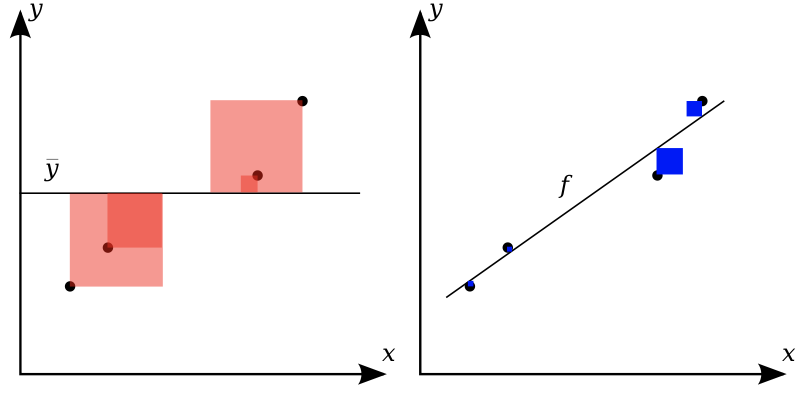
Visualizing errors
- Prediction plot (left): predicted vs actual target values
- Residual plot (right): residuals vs actual target values
- Over- and underpredictions can be given different costs
from sklearn.linear_model import Ridge
from sklearn.datasets import load_boston
boston = load_boston()

X_train, X_test, y_train, y_test = train_test_split(boston.data, boston.target)

pred = Ridge(normalize=True).fit(X_train, y_train).predict(X_test)

plt.subplot(1, 2, 1)
plt.gca().set_aspect("equal")
plt.plot([10, 50], [10, 50], '--', c='k')
plt.plot(y_test, pred, 'o', alpha=.5)
plt.ylabel("predicted")
plt.xlabel("true");

plt.subplot(1, 2, 2)
plt.gca().set_aspect("equal")
plt.plot([10, 50], [0,0], '--', c='k')
plt.plot(y_test, y_test - pred, 'o', alpha=.5)
plt.xlabel("true")
plt.ylabel("true - predicted")
plt.tight_layout();

Other considerations
- There exist techniques to correct label imbalance (see next lecture)
- Undersample the majority class, or oversample the minority class
- SMOTE (Synthetic Minority Oversampling TEchnique) adds articifial training points by interpolating existing minority class points
- Think twice before creating 'artificial' training data
- Cost-sensitive classification (not in sklearn)
- Cost matrix: a confusion matrix with a costs associated to every possible type of error
- Some algorithms allow optimizing on these costs instead of their usual loss function
- Meta-cost: builds ensemble of models by relabeling training sets to match a given cost matrix
- Black-box: can make any algorithm cost sensitive (but slower and less accurate)
- There are many more metrics to choose from
- Balanced accuracy: accuracy where each sample is weighted according to the inverse prevalence of its true class
- Identical to macro-averaged recall
- Cohen's Kappa: accuracy, taking into account the possibility of predicting the right class by chance
- 1: perfect prediction, 0: random prediction, negative: worse than random
- With $p_0$ = accuracy, and $p_e$ = accuracy of random classifier: $$\kappa = \frac{p_o - p_e}{1 - p_e}$$
- Matthews correlation coefficient: another measure that can be used on imbalanced data
- 1: perfect prediction, 0: random prediction, -1: inverse prediction $$MCC = \frac{tp \times tn - fp \times fn}{\sqrt{(tp + fp)(tp + fn)(tn + fp)(tn + fn)}}$$
- Balanced accuracy: accuracy where each sample is weighted according to the inverse prevalence of its true class
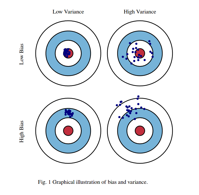
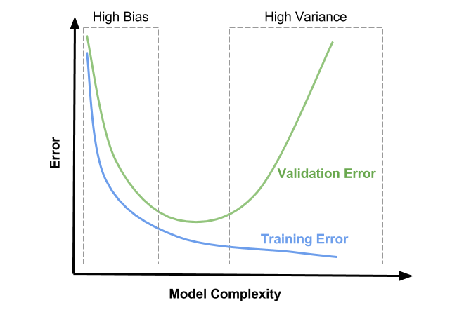
Bias-Variance decomposition
- When we repeat evaluation procedures multiple times, we can distinguish two sources of errors:
- Bias: systematic error (independent of the training sample). The classifier always gets certain points wrong
- Variance: error due to variability of the model with respect to the training sample. The classifier predicts some points accurately on some training sets, but inaccurately on others.
- There is also an intrinsic (noise) error, but there's nothing we can do against that.
- Bias is associated with underfitting, and variance with overfitting
- Bias-variance trade-off: you can often exchange variance for bias through regularization (and vice versa)
- The challenge is to find the right trade-off (minimizing total error)
- Useful to understand how to tune or adapt learning algorithm
Computing bias-variance
- Take 100 or more bootstraps (or shuffle-splits)
- Regression: for each data point x:
- $bias(x)^2 = (x_{true} - mean(x_{predicted}))^2$
- $variance(x) = var(x_{predicted})$
- Classification: for each data point x:
- $bias(x)$ = misclassification ratio
- $variance(x) = (1 - (P(class_1)^2 + P(class_2)^2))/2$
- $P(class_i)$ is ratio of class $i$ predictions
- Total bias: $\sum_{x} bias(x)^2 * w_x$, with $w_x$ the ratio of x occuring in the test sets
- Total variance: $\sum_{x} variance(x) * w_x$
Bias and variance reduction
- Bagging (RandomForests) is a variance-reduction technique
- Boosting is a bias-reduction technique
from sklearn.model_selection import ShuffleSplit, train_test_split

# Bias-Variance Computation
def compute_bias_variance(clf, X, y):
    # Bootstraps
    n_repeat = 40 # 40 is on the low side to get a good estimate. 100 is better.
    shuffle_split = ShuffleSplit(test_size=0.33, n_splits=n_repeat, random_state=0)

    # Store sample predictions
    y_all_pred = [[] for _ in range(len(y))]

    # Train classifier on each bootstrap and score predictions
    for i, (train_index, test_index) in enumerate(shuffle_split.split(X)):
        # Train and predict
        clf.fit(X[train_index], y[train_index])
        y_pred = clf.predict(X[test_index])

        # Store predictions
        for j,index in enumerate(test_index):
            y_all_pred[index].append(y_pred[j])

    # Compute bias, variance, error
    bias_sq = sum([ (1 - x.count(y[i])/len(x))**2 * len(x)/n_repeat
                for i,x in enumerate(y_all_pred)])
    var = sum([((1 - ((x.count(0)/len(x))**2 + (x.count(1)/len(x))**2))/2) * len(x)/n_repeat
               for i,x in enumerate(y_all_pred)])
    error = sum([ (1 - x.count(y[i])/len(x)) * len(x)/n_repeat
            for i,x in enumerate(y_all_pred)])

    return np.sqrt(bias_sq), var, error

from sklearn.datasets import load_breast_cancer
from sklearn.ensemble import RandomForestClassifier, AdaBoostClassifier
cancer = load_breast_cancer()

def plot_bias_variance_rf(clf, X, y):
    bias_scores = []
    var_scores = []
    err_scores = []
    n_estimators= [1, 2, 4, 8, 16, 32, 64, 128, 256]

    for i in n_estimators:
        b,v,e = compute_bias_variance(clf.set_params(random_state=0,n_estimators=i),X,y)
        bias_scores.append(b)
        var_scores.append(v)
        err_scores.append(e)

    plt.figure(figsize=(5,2))
    plt.rcParams.update({'font.size': 12})
    plt.suptitle(clf.__class__.__name__)
    plt.plot(n_estimators, var_scores,label ="variance", lw=2 )
    plt.plot(n_estimators, np.square(bias_scores),label ="bias^2", lw=2 )
    plt.plot(n_estimators, err_scores,label ="error", lw=2 )
    plt.xscale('log',basex=2)
    plt.xlabel("n_estimators")
    plt.legend(loc="best")
    plt.show()

X, y = cancer.data, cancer.target
rf = RandomForestClassifier(random_state=0, n_estimators=512, n_jobs=-1)
plot_bias_variance_rf(rf, X, y)

X, y = cancer.data, cancer.target
ab = AdaBoostClassifier(random_state=0, n_estimators=512)
plot_bias_variance_rf(ab, X, y)


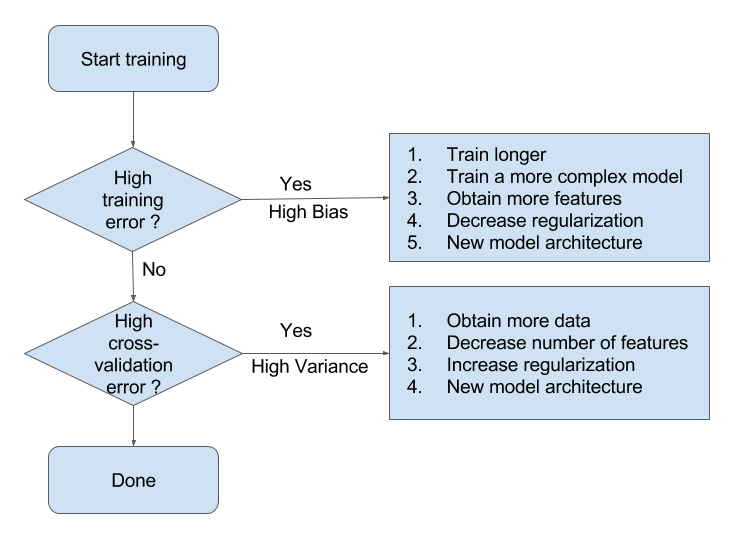
Bias-variance and overfitting
- High bias means that you are likely underfitting
- Do less regularization
- Use a more flexible/complex model (another algorithm)
- Use a bias-reduction technique (e.g. boosting)
- High variance means that you are likely overfitting
- Use more regularization
- Get more data
- Use a simpler model (another algorithm)
- Use a variance-reduction techniques (e.g. bagging)
Bias-Variance Flowchart (Andrew Ng, Coursera)
Hyperparameter tuning
We can basically use any optimization technique to optimize hyperparameters:
- Grid search
- Random search
More advanced techniques (see lecture 7):
- Local search
- Racing algorithms
- Model-based optimization (see later)
- Multi-armed bandits
- Genetic algorithms
Overfitting on the test set
- Simply taking the best performing hyperparameters yields optimistic results
- We've already used the test data to evaluate each hyperparameter setting!
- Information 'leaks' from test set into the final model
- Set aside part of the training data to evaluate the hyperparameter settings
- Select best hyperparameters on validation set
- Rebuild the model on the training+validation set
- Evaluate optimal model on the test set
mglearn.plots.plot_threefold_split()

from sklearn.svm import SVC
# split data into train+validation set and test set
X_trainval, X_test, y_trainval, y_test = train_test_split(
    iris.data, iris.target, random_state=0)
# split train+validation set into training and validation set
X_train, X_valid, y_train, y_valid = train_test_split(
    X_trainval, y_trainval, random_state=1)
print("Size of training set: {}   size of validation set: {}   size of test set:"
      " {}\n".format(X_train.shape[0], X_valid.shape[0], X_test.shape[0]))

best_score = 0

for gamma in [0.001, 0.01, 0.1, 1, 10, 100]:
    for C in [0.001, 0.01, 0.1, 1, 10, 100]:
        # for each combination of parameters
        # train an SVC
        svm = SVC(gamma=gamma, C=C)
        svm.fit(X_train, y_train)
        # evaluate the SVC on the test set
        score = svm.score(X_valid, y_valid)
        # if we got a better score, store the score and parameters
        if score > best_score:
            best_score = score
            best_parameters = {'C': C, 'gamma': gamma}

# rebuild a model on the combined training and validation set,
# and evaluate it on the test set
svm = SVC(**best_parameters)
svm.fit(X_trainval, y_trainval)
test_score = svm.score(X_test, y_test)
print("Best score on validation set: {:.2f}".format(best_score))
print("Best parameters: ", best_parameters)
print("Test set score with best parameters: {:.2f}".format(test_score))
Grid-search with cross-validation
- The way that we split the data into training, validation, and test set may have a large influence on estimated performance
- We need to use cross-validation again (e.g. 3-fold CV), instead of a single split
plt.rcParams['figure.dpi'] = 70 # Avoid overlapping boxes
mglearn.plots.plot_grid_search_overview()

Nested cross-validation
- Note that we are still using a single split to create the outer test set
- We can also use cross-validation here
- Nested cross-validation:
- Outer loop: split data in training and test sets
- Inner loop: run grid search, splitting the training data into train and validation sets
- Result is a just a list of scores
- There will be multiple optimized models and hyperparameter settings (not returned)
- To apply on future data, we need to train
GridSearchCVon all data again
scores = cross_val_score(GridSearchCV(SVC(), param_grid, cv=5),
                         iris.data, iris.target, cv=5)
scores = cross_val_score(GridSearchCV(SVC(), param_grid, cv=5),
                         iris.data, iris.target, cv=5)
print("Cross-validation scores: ", scores)
print("Mean cross-validation score: ", scores.mean())