
Lab 4: Data engineering pipelines with scikit-learn#
# Auto-setup when running on Google Colab
if 'google.colab' in str(get_ipython()):
    !pip install openml

# General imports
%matplotlib inline
import numpy as np
import pandas as pd
import matplotlib.pyplot as plt
import openml as oml
import seaborn as sns
Applying data transformations (recap from lecture)#
Data transformations should always follow a
fit-predictparadigmFitthe transformer on the training data onlyE.g. for a standard scaler: record the mean and standard deviation
Transform (e.g. scale) the training data, then train the learning model
Transform (e.g. scale) the test data, then evaluate the model
Only scale the input features (X), not the targets (y)!
If you fit and transform the whole dataset before splitting, you get data leakage
You have looked at the test data before training the model
Model evaluations will be misleading
If you fit and transform the training and test data separately, you distort the data
E.g. training and test points are scaled differently
In practice (scikit-learn)#
# choose scaling method and fit on training data
scaler = StandardScaler()
scaler.fit(X_train)

# transform training and test data
X_train_scaled = scaler.transform(X_train)
X_test_scaled = scaler.transform(X_test)
Alternative:
# calling fit and transform in sequence
X_train_scaled = scaler.fit(X_train).transform(X_train)
# same result, but more efficient computation
X_train_scaled = scaler.fit_transform(X_train)
Scikit-learn processing pipelines#
Scikit-learn pipelines have a
fit,predict, andscoremethodInternally applies transformations correctly
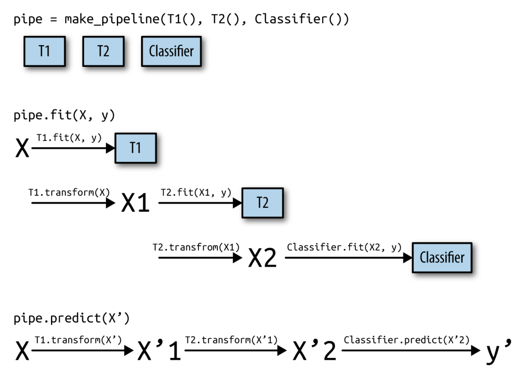
Building Pipelines#
In scikit-learn, a
pipelinecombines multiple processing steps in a single estimatorAll but the last step should be transformer (have a
transformmethod)The last step can be a transformer too (e.g. Scaler+PCA)
It has a
fit,predict, andscoremethod, just like any other learning algorithmPipelines are built as a list of steps, which are (name, algorithm) tuples
The name can be anything you want, but can’t contain
'__'We use
'__'to refer to the hyperparameters, e.g.svm__C
Let’s build, train, and score a
MinMaxScaler+LinearSVCpipeline:
pipe = Pipeline([("scaler", MinMaxScaler()), ("svm", LinearSVC())])
pipe.fit(X_train, y_train).score(X_test, y_test)
from sklearn.pipeline import Pipeline
from sklearn.preprocessing import MinMaxScaler
from sklearn.svm import LinearSVC
from sklearn.model_selection import train_test_split
from sklearn.datasets import load_breast_cancer

cancer = load_breast_cancer()
pipe = Pipeline([("scaler", MinMaxScaler()), ("svm", LinearSVC())])

X_train, X_test, y_train, y_test = train_test_split(cancer.data, cancer.target,
                                                    random_state=1)
pipe.fit(X_train, y_train)
print("Test score: {:.2f}".format(pipe.score(X_test, y_test)))
Test score: 0.97
Now with cross-validation:
scores = cross_val_score(pipe, cancer.data, cancer.target)
from sklearn.model_selection import cross_val_score
scores = cross_val_score(pipe, cancer.data, cancer.target)
print("Cross-validation scores: {}".format(scores))
print("Average cross-validation score: {:.2f}".format(scores.mean()))
Cross-validation scores: [0.98245614 0.97368421 0.96491228 0.96491228 0.99115044]
Average cross-validation score: 0.98
We can retrieve the trained SVM by querying the right step indices
pipe.steps[1][1]
pipe.fit(X_train, y_train)
print("SVM component: {}".format(pipe.steps[1][1]))
SVM component: LinearSVC()
Or we can use the
named_stepsdictionary
pipe.named_steps['svm']
print("SVM component: {}".format(pipe.named_steps['svm']))
SVM component: LinearSVC()
When you don’t need specific names for specific steps, you can use
make_pipelineAssigns names to steps automatically
pipe_short = make_pipeline(MinMaxScaler(), LinearSVC(C=100))
print("Pipeline steps:\n{}".format(pipe_short.steps))
from sklearn.pipeline import make_pipeline
# abbreviated syntax
pipe_short = make_pipeline(MinMaxScaler(), LinearSVC(C=100))
print("Pipeline steps:\n{}".format(pipe_short.steps))
Pipeline steps:
[('minmaxscaler', MinMaxScaler()), ('linearsvc', LinearSVC(C=100))]
Visualization of a pipeline fit and predict
Pipeline selection#
We can safely use pipelines in model selection (e.g. grid search)
Use
'__'to refer to the hyperparameters of a step, e.g.svm__C
# Correct grid search (can have hyperparameters of any step)
param_grid = {'svm__C': [0.001, 0.01],
              'svm__gamma': [0.001, 0.01, 0.1, 1, 10, 100]}
grid = GridSearchCV(pipe, param_grid=param_grid).fit(X,y)
# Best estimator is now the best pipeline
best_pipe = grid.best_estimator_

# Tune pipeline and evaluate on held-out test set
grid = GridSearchCV(pipe, param_grid=param_grid).fit(X_train,y_train)
grid.score(X_test,y_test)
Using Pipelines in Grid-searches#
We can use the pipeline as a single estimator in
cross_val_scoreorGridSearchCVTo define a grid, refer to the hyperparameters of the steps
Step
svm, parameterCbecomessvm__C
param_grid = {'svm__C': [0.001, 0.01, 0.1, 1, 10, 100],
              'svm__gamma': [0.001, 0.01, 0.1, 1, 10, 100]}
from sklearn import pipeline
from sklearn.svm import SVC
from sklearn.model_selection import GridSearchCV

pipe = pipeline.Pipeline([("scaler", MinMaxScaler()), ("svm", SVC(C=100))])
grid = GridSearchCV(pipe, param_grid=param_grid, cv=5)
grid.fit(X_train, y_train)
print("Best cross-validation accuracy: {:.2f}".format(grid.best_score_))
print("Test set score: {:.2f}".format(grid.score(X_test, y_test)))
print("Best parameters: {}".format(grid.best_params_))
Best cross-validation accuracy: 0.97
Test set score: 0.97
Best parameters: {'svm__C': 10, 'svm__gamma': 1}
When we request the best estimator of the grid search, we’ll get the best pipeline
grid.best_estimator_
print("Best estimator:\n{}".format(grid.best_estimator_))
Best estimator:
Pipeline(steps=[('scaler', MinMaxScaler()), ('svm', SVC(C=10, gamma=1))])
And we can drill down to individual components and their properties
grid.best_estimator_.named_steps["svm"]
# Get the SVM
print("SVM step:\n{}".format(
      grid.best_estimator_.named_steps["svm"]))
SVM step:
SVC(C=10, gamma=1)
# Get the SVM dual coefficients (support vector weights)
print("SVM support vector coefficients:\n{}".format(
      grid.best_estimator_.named_steps["svm"].dual_coef_))
SVM support vector coefficients:
[[ -1.39188844  -4.06940593  -0.435234    -0.70025696  -5.86542086
   -0.41433994  -2.81390656 -10.         -10.          -3.41806527
   -7.90768285  -0.16897821  -4.29887055  -1.13720135  -2.21362118
   -0.19026766 -10.          -7.12847723 -10.          -0.52216852
   -3.76624729  -0.01249056  -1.15920579 -10.          -0.51299862
   -0.71224989 -10.          -1.50141938 -10.          10.
    1.99516035   0.9094081    0.91913684   2.89650891   0.39896365
   10.           9.81123374   0.4124202   10.          10.
   10.           5.41518257   0.83036405   2.59337629   1.37050773
   10.           0.27947936   1.55478824   6.58895182   1.48679571
   10.           1.15559387   0.39055347   2.66341253   1.27687797
    0.65127305   1.84096369   2.39518826   2.50425662]]
Grid-searching preprocessing steps and model parameters#
We can use grid search to optimize the hyperparameters of our preprocessing steps and learning algorithms at the same time
Consider the following pipeline:
StandardScaler, without hyperparametersPolynomialFeatures, with the max. degree of polynomialsRidgeregression, with L2 regularization parameter alpha
from sklearn.datasets import fetch_california_housing
from sklearn.preprocessing import StandardScaler
from sklearn.linear_model import Ridge

housing = fetch_california_housing()
X_train, X_test, y_train, y_test = train_test_split(housing.data, housing.target,
                                                    random_state=0)
from sklearn.preprocessing import PolynomialFeatures
pipe = pipeline.make_pipeline(
    StandardScaler(),
    PolynomialFeatures(),
    Ridge())
We don’t know the optimal polynomial degree or alpha value, so we use a grid search (or random search) to find the optimal values
param_grid = {'polynomialfeatures__degree': [1, 2, 3],
              'ridge__alpha': [0.001, 0.01, 0.1, 1, 10, 100]}
grid = GridSearchCV(pipe, param_grid=param_grid, cv=5, n_jobs=1)
grid.fit(X_train, y_train)
param_grid = {'polynomialfeatures__degree': [1, 2, 3],
              'ridge__alpha': [0.001, 0.01, 0.1, 1, 10, 100]}
# Note: I had to use n_jobs=1. (n_jobs=-1 stalls on my machine)
grid = GridSearchCV(pipe, param_grid=param_grid, cv=5, n_jobs=1)
grid.fit(X_train, y_train);
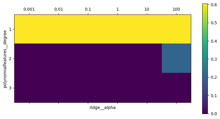
Visualing the \(R^2\) results as a heatmap:
import matplotlib.pyplot as plt

plt.matshow(grid.cv_results_['mean_test_score'].reshape(3, -1),
            vmin=0, cmap="viridis")
plt.xlabel("ridge__alpha")
plt.ylabel("polynomialfeatures__degree")
plt.xticks(range(len(param_grid['ridge__alpha'])), param_grid['ridge__alpha'])
plt.yticks(range(len(param_grid['polynomialfeatures__degree'])),
           param_grid['polynomialfeatures__degree'])

plt.colorbar();
# Another example (different dataset)

from sklearn.pipeline import make_pipeline
from sklearn.linear_model import Ridge
from sklearn.model_selection import GridSearchCV
from sklearn.datasets import fetch_openml

boston = fetch_openml(name="boston", as_frame=True)
X_train, X_test, y_train, y_test = train_test_split(boston.data, boston.target,
                                                    random_state=0)
from sklearn.preprocessing import PolynomialFeatures
pipe = make_pipeline(StandardScaler(),PolynomialFeatures(),Ridge())
param_grid = {'polynomialfeatures__degree': [1, 2, 3],
              'ridge__alpha': [0.001, 0.01, 0.1, 1, 10, 100]}
grid = GridSearchCV(pipe, param_grid=param_grid, cv=5)
grid.fit(X_train, y_train);

#plot
fig, ax = plt.subplots(figsize=(6, 3))
im = ax.matshow(grid.cv_results_['mean_test_score'].reshape(3, -1),
            vmin=0, cmap="viridis")
ax.set_xlabel("ridge__alpha")
ax.set_ylabel("polynomialfeatures__degree")
ax.set_xticks(range(len(param_grid['ridge__alpha'])))
ax.set_xticklabels(param_grid['ridge__alpha'])
ax.set_yticks(range(len(param_grid['polynomialfeatures__degree'])))
ax.set_yticklabels(param_grid['polynomialfeatures__degree'])
plt.colorbar(im);
/Users/jvanscho/miniconda3/envs/mlcourse/lib/python3.10/site-packages/sklearn/datasets/_openml.py:323: UserWarning: Multiple active versions of the dataset matching the name boston exist. Versions may be fundamentally different, returning version 1. Available versions:
- version 1, status: active
  url: https://www.openml.org/search?type=data&id=531
- version 2, status: active
  url: https://www.openml.org/search?type=data&id=853

  warn(warning_msg)
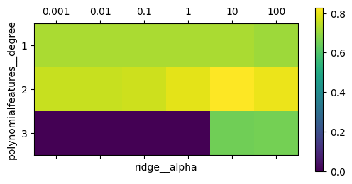
Here, degree-2 polynomials help (but degree-3 ones don’t), and tuning the alpha parameter helps as well.
Not using the polynomial features leads to suboptimal results (see the results for degree 1)
print("Best parameters: {}".format(grid.best_params_))
print("Test-set score: {:.2f}".format(grid.score(X_test, y_test)))
Best parameters: {'polynomialfeatures__degree': 2, 'ridge__alpha': 10}
Test-set score: 0.77
FeatureUnions#
Sometimes you want to apply multiple preprocessing techniques and use the combined produced features
Simply appending the produced features is called a
FeatureJoinExample: Apply both PCA and feature selection, and run an SVM on both
from sklearn.pipeline import Pipeline, FeatureUnion
from sklearn.svm import SVC
from sklearn.datasets import load_iris
from sklearn.decomposition import PCA
from sklearn.feature_selection import SelectKBest

iris = load_iris()

X, y = iris.data, iris.target

# This dataset is way too high-dimensional. Better do PCA:
pca = PCA(n_components=2)

# Maybe some original features where good, too?
selection = SelectKBest(k=1)

# Build estimator from PCA and Univariate selection:

combined_features = FeatureUnion([("pca", pca), ("univ_select", selection)])

# Use combined features to transform dataset:
X_features = combined_features.fit(X, y).transform(X)
print("Combined space has", X_features.shape[1], "features")

svm = SVC(kernel="linear")

# Do grid search over k, n_components and C:

pipeline = Pipeline([("features", combined_features), ("svm", svm)])

param_grid = dict(features__pca__n_components=[1, 2, 3],
                  features__univ_select__k=[1, 2],
                  svm__C=[0.1, 1, 10])

grid_search = GridSearchCV(pipeline, param_grid=param_grid)
grid_search.fit(X, y)
print(grid_search.best_estimator_)
Combined space has 3 features
Pipeline(steps=[('features',
                 FeatureUnion(transformer_list=[('pca', PCA(n_components=3)),
                                                ('univ_select',
                                                 SelectKBest(k=1))])),
                ('svm', SVC(C=10, kernel='linear'))])
ColumnTransformer#
A pipeline applies a transformer on all columns
If your dataset has both numeric and categorical features, you often want to apply different techniques on each
You could manually split up the dataset, and then feature-join the processed features (tedious)
ColumnTransformerallows you to specify on which columns a preprocessor has to be runEither by specifying the feature names, indices, or a binary mask
You can include multiple transformers in a ColumnTransformer
In the end the results will be feature-joined
Hence, the order of the features will change! The features of the last transformer will be at the end
Each transformer can be a pipeline
Handy if you need to apply multiple preprocessing steps on a set of features
E.g. use a ColumnTransformer with one sub-pipeline for numerical features and one for categorical features.
In the end, the columntransformer can again be included as part of a pipeline
E.g. to add a classfier and include the whole pipeline in a grid search
# 2 sub-pipelines, one for numeric features, other for categorical ones
numeric_pipe = make_pipeline(SimpleImputer(),StandardScaler())
categorical_pipe = make_pipeline(SimpleImputer(),OneHotEncoder())

# Using categorical pipe for features A,B,C, numeric pipe otherwise
preprocessor = make_column_transformer((categorical_pipe,
                                        ["A","B","C"]),
                                        remainder=numeric_pipe)

# Combine with learning algorithm in another pipeline

``` python
pipe = make_pipeline(preprocessor, LinearSVC())
Careful:
ColumnTransformerconcatenates features in order
pipe = make_column_transformer((StandardScaler(),numeric_features),
                               (PCA(),numeric_features),
                               (OneHotEncoder(),categorical_features))
Example: Handle a dataset (Titanic) with both categorical an numeric features
Numeric features: impute missing values and scale
Categorical features: Impute missing values and apply one-hot-encoding
Finally, run an SVM
from sklearn.compose import ColumnTransformer
from sklearn.datasets import fetch_openml
from sklearn.impute import SimpleImputer
from sklearn.preprocessing import StandardScaler, OneHotEncoder
from sklearn.linear_model import LogisticRegression
from sklearn.model_selection import train_test_split, GridSearchCV

np.random.seed(0)

# Load data from https://www.openml.org/d/40945
X, y = fetch_openml("titanic", version=1, as_frame=True, return_X_y=True)

# Alternatively X and y can be obtained directly from the frame attribute:
# X = titanic.frame.drop('survived', axis=1)
# y = titanic.frame['survived']

# We will train our classifier with the following features:
# Numeric Features:
# - age: float.
# - fare: float.
# Categorical Features:
# - embarked: categories encoded as strings {'C', 'S', 'Q'}.
# - sex: categories encoded as strings {'female', 'male'}.
# - pclass: ordinal integers {1, 2, 3}.

# We create the preprocessing pipelines for both numeric and categorical data.
numeric_features = ['age', 'fare']
numeric_transformer = Pipeline(steps=[
    ('imputer', SimpleImputer(strategy='median')),
    ('scaler', StandardScaler())])

categorical_features = ['embarked', 'sex', 'pclass']
categorical_transformer = Pipeline(steps=[
    ('imputer', SimpleImputer(strategy='constant', fill_value='missing')),
    ('onehot', OneHotEncoder(handle_unknown='ignore'))])

preprocessor = ColumnTransformer(
    transformers=[
        ('num', numeric_transformer, numeric_features),
        ('cat', categorical_transformer, categorical_features)])

# Append classifier to preprocessing pipeline.
# Now we have a full prediction pipeline.
clf = Pipeline(steps=[('preprocessor', preprocessor),
                      ('classifier', LogisticRegression())])

X_train, X_test, y_train, y_test = train_test_split(X, y, test_size=0.2)

clf.fit(X_train, y_train)
print("model score: %.3f" % clf.score(X_test, y_test))
model score: 0.790
You can again run optimize any of the hyperparameters (preprocessing-related ones included) in a grid search
param_grid = {
    'preprocessor__num__imputer__strategy': ['mean', 'median'],
    'classifier__C': [0.1, 1.0, 10, 100],
}

grid_search = GridSearchCV(clf, param_grid, cv=10)
grid_search.fit(X_train, y_train)

print(("best logistic regression from grid search: %.3f"
       % grid_search.score(X_test, y_test)))
best logistic regression from grid search: 0.798