Lecture 6. Neural Networks

Lecture 6. Neural Networks#

How to train your neurons

Joaquin Vanschoren

Overview#

Neural architectures
Training neural nets
- Forward pass: Tensor operations
- Backward pass: Backpropagation
Neural network design:
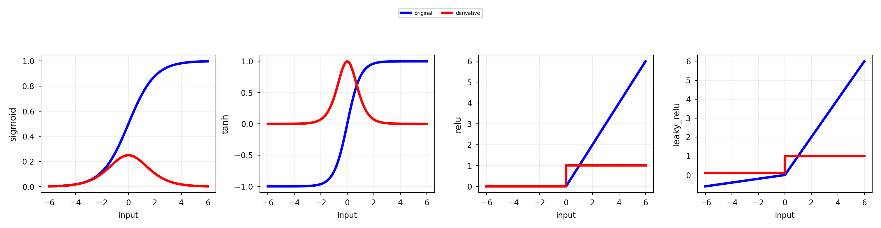
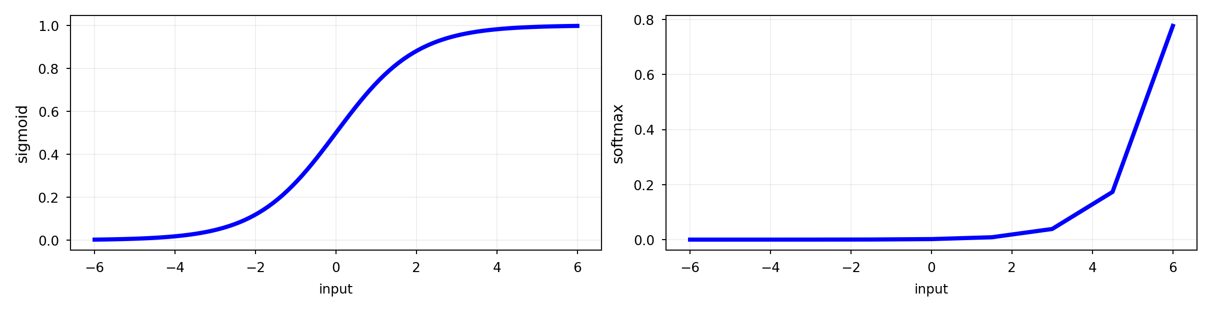
- Activation functions
- Weight initialization
- Optimizers
Neural networks in practice
Model selection
- Early stopping
- Memorization capacity and information bottleneck
- L1/L2 regularization
- Dropout
- Batch normalization

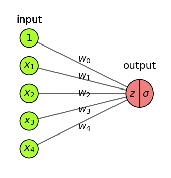
Architecture#

Logistic regression, drawn in a different, neuro-inspired, way
- Linear model: inner product ($z$) of input vector $\mathbf{x}$ and weight vector $\mathbf{w}$, plus bias $w_0$
- Logistic (or sigmoid) function maps the output to a probability in [0,1]
- Uses log loss (cross-entropy) and gradient descent to learn the weights

\[\hat{y}(\mathbf{x}) = \text{sigmoid}(z) = \text{sigmoid}(w_0 + \mathbf{w}\mathbf{x}) = \text{sigmoid}(w_0 + w_1 * x_1 + w_2 * x_2 +... + w_p * x_p)\]

../_images/9ff8adaf13b2e98a72d0ae725bfe67cc0bcef299cb6ebdbc7c906740ba66e99b.png

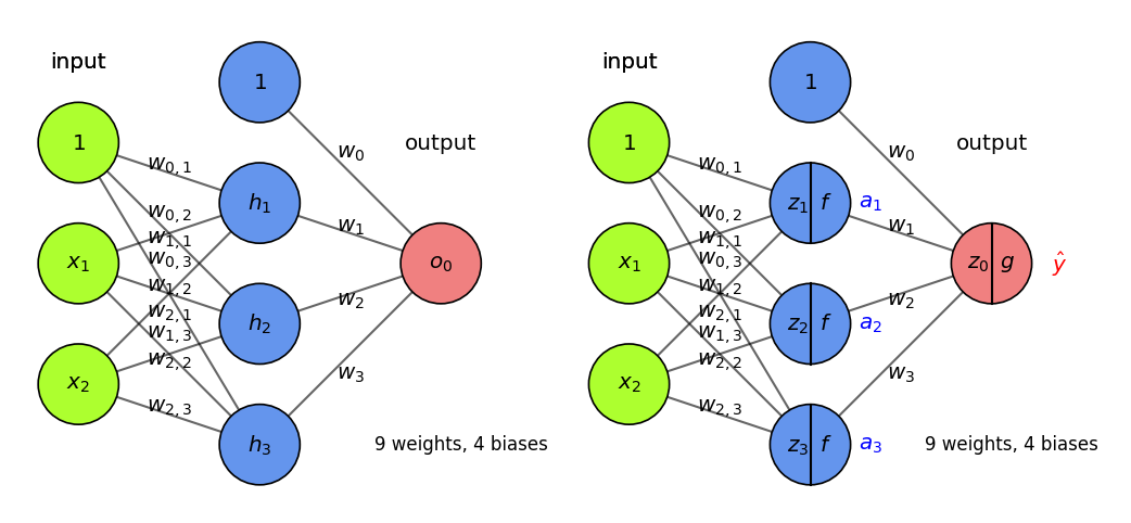
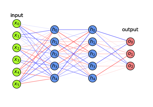
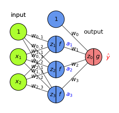
Basic Architecture#

Add one (or more) hidden layers $h$ with $k$ nodes (or units, cells, neurons)
- Every ‘neuron’ is a tiny function, the network is an arbitrarily complex function
- Weights $w_{i,j}$ between node $i$ and node $j$ form a weight matrix $\mathbf{W}^{(l)}$ per layer $l$
Every neuron weights the inputs $\mathbf{x}$ and passes it through a non-linear activation function
- Activation functions ($f,g$) can be different per layer, output $\mathbf{a}$ is called activation $$\color{blue}{h(\mathbf{x})} = \color{blue}{\mathbf{a}} = f(\mathbf{z}) = f(\mathbf{W}^{(1)} \color{green}{\mathbf{x}}+\mathbf{w}^{(1)}_0) \quad \quad \color{red}{o(\mathbf{x})} = g(\mathbf{W}^{(2)} \color{blue}{\mathbf{a}}+\mathbf{w}^{(2)}_0)$$

../_images/f1b83b78fa150b801053748afccbbecc8ae71fa127ad5a57819db6de5f9f6097.png

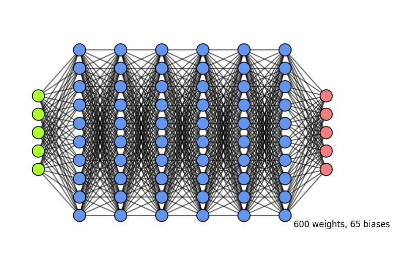
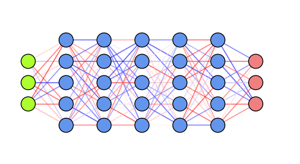
More layers#

Add more layers, and more nodes per layer, to make the model more complex
- For simplicity, we don’t draw the biases (but remember that they are there)
In dense (fully-connected) layers, every previous layer node is connected to all nodes
The output layer can also have multiple nodes (e.g. 1 per class in multi-class classification)

../_images/39538afb543359cf8768def5998551bb4396d3977c10c5f370f04db1306100ae.png

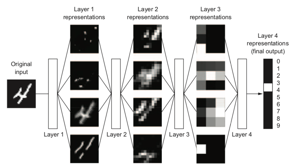
Why layers?#

Each layer acts as a filter and learns a new representation of the data
- Subsequent layers can learn iterative refinements
- Easier than learning a complex relationship in one go
Example: for image input, each layer yields new (filtered) images
- Can learn multiple mappings at once: weight tensor $\mathit{W}$ yields activation tensor $\mathit{A}$
- From low-level patterns (edges, end-points, …) to combinations thereof
- Each neuron ‘lights up’ if certain patterns occur in the input

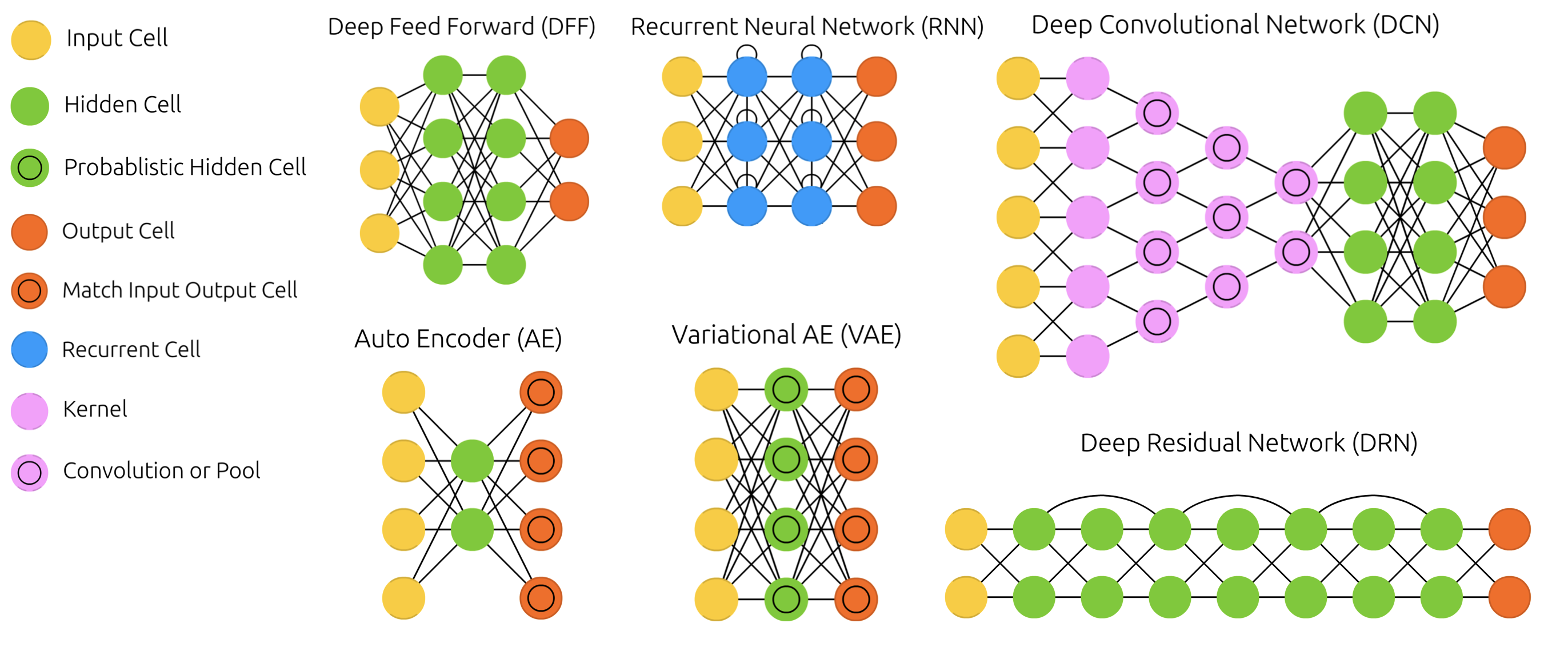
Other architectures#

There exist MANY types of networks for many different tasks
Convolutional nets for image data, Recurrent nets for sequential data,…
Also used to learn representations (embeddings), generate new images, text,…

Training Neural Nets#

Design the architecture, choose activation functions (e.g. sigmoids)
Choose a way to initialize the weights (e.g. random initialization)
Choose a loss function (e.g. log loss) to measure how well the model fits training data
Choose an optimizer (typically an SGD variant) to update the weights

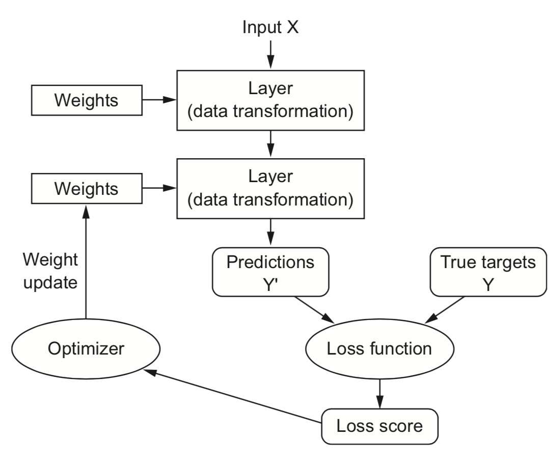
Mini-batch Stochastic Gradient Descent (recap)#

Draw a batch of batch_size training data $\mathbf{X}$ and $\mathbf{y}$
Forward pass : pass $\mathbf{X}$ though the network to yield predictions $\mathbf{\hat{y}}$
Compute the loss $\mathcal{L}$ (mismatch between $\mathbf{\hat{y}}$ and $\mathbf{y}$)
Backward pass : Compute the gradient of the loss with regard to every weight
- Backpropagate the gradients through all the layers
Update $W$: $W_{(i+1)} = W_{(i)} - \frac{\partial L(x, W_{(i)})}{\partial W} * \eta$

Repeat until n passes (epochs) are made through the entire training set

../_images/ac21e2f7e5627c4fc9eccb6b9593a5b7c9b8acd0593e11ddcfd85645069202fc.png

Forward pass#

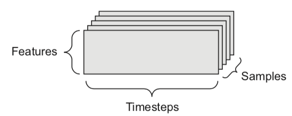
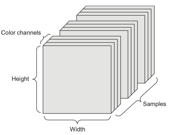
We can naturally represent the data as tensors
- Numerical n-dimensional array (with n axes)
- 2D tensor: matrix (samples, features)
- 3D tensor: time series (samples, timesteps, features)
- 4D tensor: color images (samples, height, width, channels)
- 5D tensor: video (samples, frames, height, width, channels)

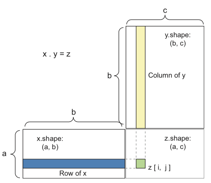
Tensor operations#

The operations that the network performs on the data can be reduced to a series of tensor operations
- These are also much easier to run on GPUs
A dense layer with sigmoid activation, input tensor $\mathbf{X}$, weight tensor $\mathbf{W}$, bias $\mathbf{b}$:

y = sigmoid(np.dot(X, W) + b)

Tensor dot product for 2D inputs ($a$ samples, $b$ features, $c$ hidden nodes)

Element-wise operations#

Activation functions and addition are element-wise operations:

def sigmoid(x):
  return 1/(1 + np.exp(-x)) 

def add(x, y):
  return x + y

Note: if y has a lower dimension than x, it will be broadcasted: axes are added to match the dimensionality, and y is repeated along the new axes

>>> np.array([[1,2],[3,4]]) + np.array([10,20])
array([[11, 22],
       [13, 24]])

Backward pass (backpropagation)#

For last layer, compute gradient of the loss function $\mathcal{L}$ w.r.t all weights of layer $l$

\[\begin{split}\nabla \mathcal{L} = \frac{\partial \mathcal{L}}{\partial W^{(l)}} = \begin{bmatrix} \frac{\partial \mathcal{L}}{\partial w_{0,0}} & \ldots & \frac{\partial \mathcal{L}}{\partial w_{0,l}} \\ \vdots & \ddots & \vdots \\ \frac{\partial \mathcal{L}}{\partial w_{k,0}} & \ldots & \frac{\partial \mathcal{L}}{\partial w_{k,l}} \end{bmatrix}\end{split}\]

Sum up the gradients for all $\mathbf{x}_j$ in minibatch: $\sum_{j} \frac{\partial \mathcal{L}(\mathbf{x}_j,y_j)}{\partial W^{(l)}}$
Update all weights in a layer at once (with learning rate $\eta$): $W_{(i+1)}^{(l)} = W_{(i)}^{(l)} - \eta \sum_{j} \frac{\partial \mathcal{L}(\mathbf{x}_j,y_j)}{\partial W_{(i)}^{(l)}}$
Repeat for next layer, iterating backwards (most efficient, avoids redundant calculations)

Example#

Imagine feeding a single data point, output is $\hat{y} = g(z) = g(w_0 + w_1 * a_1 + w_2 * a_2 +... + w_p * a_p)$
Decrease loss by updating weights:
- Update the weights of last layer to maximize improvement: $w_{i,(new)} = w_{i} - \frac{\partial \mathcal{L}}{\partial w_i} * \eta$
- To compute gradient $\frac{\partial \mathcal{L}}{\partial w_i}$ we need the chain rule: $f(g(x)) = f'(g(x)) * g'(x)$ $$\frac{\partial \mathcal{L}}{\partial w_i} = \color{red}{\frac{\partial \mathcal{L}}{\partial g}} \color{blue}{\frac{\partial \mathcal{g}}{\partial z_0}} \color{green}{\frac{\partial \mathcal{z_0}}{\partial w_i}}$$
E.g., with $\mathcal{L} = \frac{1}{2}(y-\hat{y})^2$ and sigmoid $\sigma$: $\frac{\partial \mathcal{L}}{\partial w_i} = \color{red}{(y - \hat{y})} * \color{blue}{\sigma'(z_0)} * \color{green}{a_i}$

../_images/7f33ddaf0424bbdd24aea0076e722930175bca525f7dcf01dfe22f11d7e9a35d.png

Backpropagation (2)#

Another way to decrease the loss $\mathcal{L}$ is to update the activations $a_i$
- To update $a_i = f(z_i)$, we need to update the weights of the previous layer
- We want to nudge $a_i$ in the right direction by updating $w_{i,j}$: $$\frac{\partial \mathcal{L}}{\partial w_{i,j}} = \frac{\partial \mathcal{L}}{\partial a_i} \frac{\partial a_i}{\partial z_i} \frac{\partial \mathcal{z_i}}{\partial w_{i,j}} = \left( \frac{\partial \mathcal{L}}{\partial g} \frac{\partial \mathcal{g}}{\partial z_0} \frac{\partial \mathcal{z_0}}{\partial a_i} \right) \frac{\partial a_i}{\partial z_i} \frac{\partial \mathcal{z_i}}{\partial w_{i,j}}$$
- We know $\frac{\partial \mathcal{L}}{\partial g}$ and $\frac{\partial \mathcal{g}}{\partial z_0}$ from the previous step, $\frac{\partial \mathcal{z_0}}{\partial a_i} = w_i$, $\frac{\partial a_i}{\partial z_i} = f'$ and $\frac{\partial \mathcal{z_i}}{\partial w_{i,j}} = x_j$

../_images/6410abf6583967aa6cfe329c78e6b4b283b3561049807da1eb7ab2c0ef011753.png

Backpropagation (3)#

With multiple output nodes, $\mathcal{L}$ is the sum of all per-output (per-class) losses
- $\frac{\partial \mathcal{L}}{\partial a_i}$ is sum of the gradients for every output
Per layer, sum up gradients for every point $\mathbf{x}$ in the batch: $\sum_{j} \frac{\partial \mathcal{L}(\mathbf{x}_j,y_j)}{\partial W}$
Update all weights of every layer $l$
- $W_{(i+1)}^{(l)} = W_{(i)}^{(l)} - \eta \sum_{j} \frac{\partial \mathcal{L}(\mathbf{x}_j,y_j)}{\partial W_{(i)}^{(l)}}$
Repeat with a new batch of data until loss converges
Nice animation of the entire process

../_images/ec362906f18a38f65157554ce88e629c7aa708c8eb8f4667ac2275c8d8b3d703.png

Summary#

The network output $a_o$ is defined by the weights $W^{(o)}$ and biases $\mathbf{b}^{(o)}$ of the output layer, and
The activations of a hidden layer $h_1$ with activation function $a_{h_1}$, weights $W^{(1)}$ and biases $\mathbf{b^{(1)}}$:

\[\color{red}{a_o(\mathbf{x})} = \color{red}{a_o(\mathbf{z_0})} = \color{red}{a_o(W^{(o)}} \color{blue}{a_{h_1}(z_{h_1})} \color{red}{+ \mathbf{b}^{(o)})} = \color{red}{a_o(W^{(o)}} \color{blue}{a_{h_1}(W^{(1)} \color{green}{\mathbf{x}} + \mathbf{b}^{(1)})} \color{red}{+ \mathbf{b}^{(o)})} \]

Minimize the loss by SGD. For layer $l$, compute $\frac{\partial \mathcal{L}(a_o(x))}{\partial W_l}$ and $\frac{\partial \mathcal{L}(a_o(x))}{\partial b_{l,i}}$ using the chain rule
Decomposes into gradient of layer above, gradient of activation function, gradient of layer input:

\[\frac{\partial \mathcal{L}(a_o)}{\partial W^{(1)}} = \color{red}{\frac{\partial \mathcal{L}(a_o)}{\partial a_{h_1}}} \color{blue}{\frac{\partial a_{h_1}}{\partial z_{h_1}}} \color{green}{\frac{\partial z_{h_1}}{\partial W^{(1)}}} = \left( \color{red}{\frac{\partial \mathcal{L}(a_o)}{\partial a_o}} \color{blue}{\frac{\partial a_o}{\partial z_o}} \color{green}{\frac{\partial z_o}{\partial a_{h_1}}}\right) \color{blue}{\frac{\partial a_{h_1}}{\partial z_{h_1}}} \color{green}{\frac{\partial z_{h_1}}{\partial W^{(1)}}} \]

Activation functions for hidden layers#

Sigmoid: $f(z) = \frac{1}{1+e^{-z}}$
Tanh: $f(z) = \frac{2}{1+e^{-2z}} - 1$
- Activations around 0 are better for gradient descent convergence
Rectified Linear (ReLU): $f(z) = max(0,z)$
- Less smooth, but much faster (note: not differentiable at 0)
Leaky ReLU: $f(z) = \begin{cases} 0.01z & z<0 \\ z & otherwise \end{cases}$

Show code cell source Hide code cell source

def activation(X, function="sigmoid"):     
    if function == "sigmoid":      
        return 1.0/(1.0 + np.exp(-X))    
    if function == "softmax": 
        return np.exp(X) / np.sum(np.exp(X), axis=0)   
    elif function == "tanh":      
        return np.tanh(X)    
    elif function == "relu":      
        return np.maximum(0,X)    
    elif function == "leaky_relu":      
        return np.maximum(0.1*X,X)
    elif function == "none":      
        return X
    
def activation_derivative(X, function="sigmoid"):   
    if function == "sigmoid": 
        sig = 1.0/(1.0 + np.exp(-X))   
        return sig * (1 - sig)
    elif function == "tanh":      
        return 1 - np.tanh(X)**2   
    elif function == "relu":      
        return np.where(X > 0, 1, 0)
    elif function == "leaky_relu":    
        # Using 0.1 instead of 0.01 to make it visible in the plot
        return np.where(X > 0, 1, 0.1)
    elif function == "none":      
        return X/X
    
def plot_activation(function, ax, derivative=False):
    if function=="softmax":       
        x = np.linspace(-6,6,9)
        ax.plot(x,activation(x, function),lw=2, c='b', linestyle='-', marker='o')
    else:     
        x = np.linspace(-6,6,101)
        ax.plot(x,activation(x, function),lw=2, c='b', linestyle='-') 
        if derivative:
            if function == "relu" or function == "leaky_relu":
                ax.step(x,activation_derivative(x, function),lw=2, c='r', linestyle='-')
            else:
                ax.plot(x,activation_derivative(x, function),lw=2, c='r', linestyle='-')
    ax.set_xlabel("input", fontsize=16*fig_scale)
    ax.set_ylabel(function, fontsize=18*fig_scale)
    ax.tick_params(axis='both', labelsize=16*fig_scale)
    ax.grid()
    
functions = ["sigmoid","tanh","relu","leaky_relu"]

@interact
def plot_activations(function=functions):
    fig, ax = plt.subplots(figsize=(5,1.5))
    plot_activation(function, ax)
    plt.show()

../_images/d735e76d44fe3db245923b7a2cb753338bbafc6d1b71fc4c081cbd865f06a348.png

Effect of activation functions on the gradient#

During gradient descent, the gradient depends on the activation function $a_{h}$: $\frac{\partial \mathcal{L}(a_o)}{\partial W^{(l)}} = \color{red}{\frac{\partial \mathcal{L}(a_o)}{\partial a_{h_l}}} \color{blue}{\frac{\partial a_{h_l}}{\partial z_{h_l}}} \color{green}{\frac{\partial z_{h_l}}{\partial W^{(l)}}}$
If derivative of the activation function $\color{blue}{\frac{\partial a_{h_l}}{\partial z_{h_l}}}$ is 0, the weights $w_i$ are not updated
- Moreover, the gradients of previous layers will be reduced (vanishing gradient)
sigmoid, tanh: gradient is very small for large inputs: slow updates
With ReLU, $\color{blue}{\frac{\partial a_{h_l}}{\partial z_{h_l}}} = 1$ if $z>0$, hence better against vanishing gradients
- Problem: for very negative inputs, the gradient is 0 and may never recover (dying ReLU)
- Leaky ReLU has a small (0.01) gradient there to allow recovery

../_images/c53fc05c1577c4cd4f399c80d37ce2d7458603138743d48cbe4b468452c37bb6.png

ReLU vs Tanh#

What is the effect of using non-smooth activation functions?
- ReLU produces piecewise-linear boundaries, but allows deeper networks
- Tanh produces smoother decision boundaries, but is slower

../_images/df30627dd0a20f6214070762c0909a252583a675c91faa617227320b632db8b7.png

Activation functions for output layer#

sigmoid converts output to probability in [0,1]
- For binary classification
softmax converts all outputs (aka ‘logits’) to probabilities that sum up to 1
- For multi-class classification ($k$ classes)
- Can cause over-confident models. If so, smooth the labels: $y_{smooth} = (1-\alpha)y + \frac{\alpha}{k}$ $$\text{softmax}(\mathbf{x},i) = \frac{e^{x_i}}{\sum_{j=1}^k e^{x_j}}$$
For regression, don’t use any activation function, let the model learn the exact target

../_images/9a5ec41d73ecc4d3074b0e4fbf24e34509af0a20269aa0c48c8ceef0a39a9d56.png

Weight initialization#

Initializing weights to 0 is bad: all gradients in layer will be identical (symmetry)
Too small random weights shrink activations to 0 along the layers (vanishing gradient)
Too large random weights multiply along layers (exploding gradient, zig-zagging)
Ideal: small random weights + variance of input and output gradients remains the same
- Glorot/Xavier initialization (for tanh): randomly sample from $N(0,\sigma), \sigma = \sqrt{\frac{2}{\text{fan_in + fan_out}}}$
  - fan_in: number of input units, fan_out: number of output units
- He initialization (for ReLU): randomly sample from $N(0,\sigma), \sigma = \sqrt{\frac{2}{\text{fan_in}}}$
- Uniform sampling (instead of $N(0,\sigma)$) for deeper networks (w.r.t. vanishing gradients)

../_images/4d186b04063cb77d8f146bad433f162d0054a9ebe7dddae82adc50e3ac19d0b9.png

Weight initialization: transfer learning#

Instead of starting from scratch, start from weights previously learned from similar tasks
- This is, to a big extent, how humans learn so fast
Transfer learning: learn weights on task T, transfer them to new network
- Weights can be frozen, or finetuned to the new data
Only works if the previous task is ‘similar’ enough
- Generally, weights learned on very diverse data (e.g. ImageNet) transfer better
- Meta-learning: learn a good initialization across many related tasks

import tensorflow as tf
#import tensorflow_addons as tfa

# Toy surface
def f(x, y):
    return (1.5 - x + x*y)**2 + (2.25 - x + x*y**2)**2 + (2.625 - x + x*y**3)**2

# Tensorflow optimizers
class CyclicalLearningRate(tf.keras.optimizers.schedules.LearningRateSchedule):
    def __init__(self, initial_learning_rate, maximal_learning_rate, step_size):
        self.initial_learning_rate = initial_learning_rate
        self.maximal_learning_rate = maximal_learning_rate
        self.step_size = step_size

    def __call__(self, step):
        cycle = tf.floor(1 + step / (2 * self.step_size))
        x = tf.abs(step / self.step_size - 2 * cycle + 1)
        return self.initial_learning_rate + (self.maximal_learning_rate - self.initial_learning_rate) * tf.maximum(0.0, (1 - x))

clr_schedule = CyclicalLearningRate(initial_learning_rate=1e-4, 
                                    maximal_learning_rate=0.1, 
                                    step_size=100)
sgd_cyclic = tf.keras.optimizers.SGD(learning_rate=clr_schedule)
sgd = tf.optimizers.SGD(0.01)
lr_schedule = tf.optimizers.schedules.ExponentialDecay(0.02,decay_steps=100,decay_rate=0.96)
sgd_decay = tf.optimizers.SGD(learning_rate=lr_schedule)
momentum = tf.optimizers.SGD(0.005, momentum=0.9, nesterov=False)
nesterov = tf.optimizers.SGD(0.005, momentum=0.9, nesterov=True)
adagrad = tf.optimizers.Adagrad(0.4)
rmsprop = tf.optimizers.RMSprop(learning_rate=0.1)
adam = tf.optimizers.Adam(learning_rate=0.2, beta_1=0.9, beta_2=0.999, epsilon=1e-8)

optimizers = [sgd, sgd_decay, momentum, nesterov, adagrad, rmsprop, adam, sgd_cyclic]
opt_names = ['sgd', 'sgd_decay', 'momentum', 'nesterov', 'adagrad', 'rmsprop', 'adam', 'sgd_cyclic']
cmap = plt.cm.get_cmap('tab10')
colors = [cmap(x/10) for x in range(10)]

# Training
all_paths = []
for opt, name in zip(optimizers, opt_names):
    x = tf.Variable(0.8)
    y = tf.Variable(1.6)

    x_history = []
    y_history = []
    loss_prev = 0.0
    max_steps = 100
    for step in range(max_steps):
        with tf.GradientTape() as g:
            loss = f(x, y)
            x_history.append(x.numpy())
            y_history.append(y.numpy())
            grads = g.gradient(loss, [x, y])
            opt.apply_gradients(zip(grads, [x, y]))

    if np.abs(loss_prev - loss.numpy()) < 1e-6:
        break
    loss_prev = loss.numpy()
    x_history = np.array(x_history)
    y_history = np.array(y_history)
    path = np.concatenate((np.expand_dims(x_history, 1), np.expand_dims(y_history, 1)), axis=1).T
    all_paths.append(path)

# Plotting
number_of_points = 50
margin = 4.5
minima = np.array([3., .5])
minima_ = minima.reshape(-1, 1)
x_min = 0. - 2
x_max = 0. + 3.5
y_min = 0. - 3.5
y_max = 0. + 2
x_points = np.linspace(x_min, x_max, number_of_points) 
y_points = np.linspace(y_min, y_max, number_of_points)
x_mesh, y_mesh = np.meshgrid(x_points, y_points)
z = np.array([f(xps, yps) for xps, yps in zip(x_mesh, y_mesh)])

def plot_optimizers(ax, iterations, optimizers):
    ax.contour(x_mesh, y_mesh, z, levels=np.logspace(-0.5, 5, 25), norm=LogNorm(), cmap=plt.cm.jet, linewidths=fig_scale, zorder=-1)
    ax.plot(*minima, 'r*', markersize=20*fig_scale)
    for name, path, color in zip(opt_names, all_paths, colors):
        if name in optimizers:
            p = path[:,:iterations]
            ax.plot([], [], color=color, label=name, lw=3*fig_scale, linestyle='-')
            ax.quiver(p[0,:-1], p[1,:-1], p[0,1:]-p[0,:-1], p[1,1:]-p[1,:-1], scale_units='xy', angles='xy', scale=1, color=color, lw=4)


    ax.set_xlim((x_min, x_max))
    ax.set_ylim((y_min, y_max))
    ax.legend(loc='lower left', prop={'size': 15*fig_scale}) 
    ax.set_xticks([])
    ax.set_yticks([])
    plt.tight_layout()

from decimal import *
from matplotlib.colors import LogNorm

# Training for momentum
all_lr_paths = []
lr_range = [0.005 * i for i in range(0,10)]
for lr in lr_range:
    opt = tf.optimizers.SGD(lr, nesterov=False)

    x_init = 0.8
    x = tf.compat.v1.get_variable('x', dtype=tf.float32, initializer=tf.constant(x_init))
    y_init = 1.6
    y = tf.compat.v1.get_variable('y', dtype=tf.float32, initializer=tf.constant(y_init))

    x_history = []
    y_history = []
    z_prev = 0.0
    max_steps = 100
    for step in range(max_steps):
        with tf.GradientTape() as g:
            z = f(x, y)
            x_history.append(x.numpy())
            y_history.append(y.numpy())
            dz_dx, dz_dy = g.gradient(z, [x, y])
            opt.apply_gradients(zip([dz_dx, dz_dy], [x, y]))

    if np.abs(z_prev - z.numpy()) < 1e-6:
        break
    z_prev = z.numpy()
    x_history = np.array(x_history)
    y_history = np.array(y_history)
    path = np.concatenate((np.expand_dims(x_history, 1), np.expand_dims(y_history, 1)), axis=1).T
    all_lr_paths.append(path)
    
# Plotting
number_of_points = 50
margin = 4.5
minima = np.array([3., .5])
minima_ = minima.reshape(-1, 1)
x_min = 0. - 2
x_max = 0. + 3.5
y_min = 0. - 3.5
y_max = 0. + 2
x_points = np.linspace(x_min, x_max, number_of_points) 
y_points = np.linspace(y_min, y_max, number_of_points)
x_mesh, y_mesh = np.meshgrid(x_points, y_points)
z = np.array([f(xps, yps) for xps, yps in zip(x_mesh, y_mesh)])

def plot_learning_rate_optimizers(ax, iterations, lr):
    ax.contour(x_mesh, y_mesh, z, levels=np.logspace(-0.5, 5, 25), norm=LogNorm(), cmap=plt.cm.jet, linewidths=fig_scale, zorder=-1)
    ax.plot(*minima, 'r*', markersize=20*fig_scale)
    for path, lrate in zip(all_lr_paths, lr_range):
        if round(lrate,3) == lr:
            p = path[:,:iterations]
            ax.plot([], [], color='b', label="Learning rate {}".format(lr), lw=3*fig_scale, linestyle='-')
            ax.quiver(p[0,:-1], p[1,:-1], p[0,1:]-p[0,:-1], p[1,1:]-p[1,:-1], scale_units='xy', angles='xy', scale=1, color='b', lw=4)


    ax.set_xlim((x_min, x_max))
    ax.set_ylim((y_min, y_max))
    ax.legend(loc='lower left', prop={'size': 15*fig_scale}) 
    ax.set_xticks([])
    ax.set_yticks([])
    plt.tight_layout()

Optimizers#

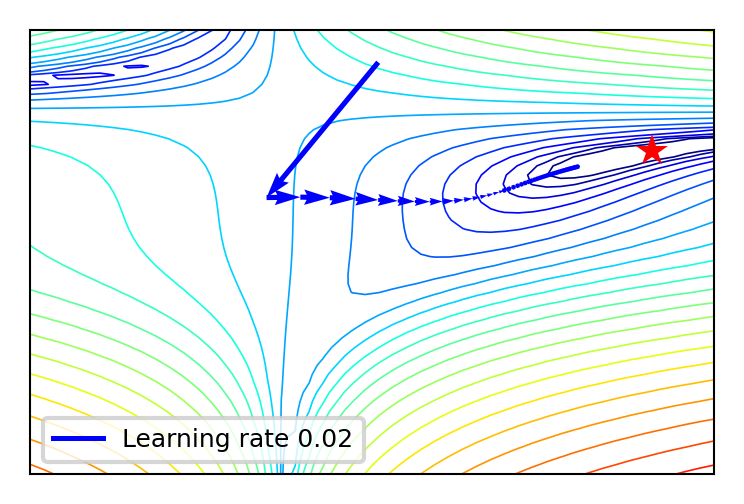
SGD with learning rate schedules#

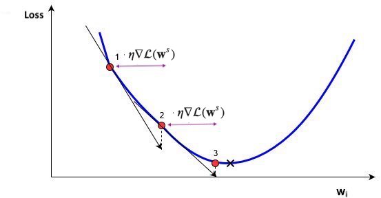
Using a constant learning $\eta$ rate for weight updates $\mathbf{w}_{(s+1)} = \mathbf{w}_s-\eta\nabla \mathcal{L}(\mathbf{w}_s)$ is not ideal
- You would need to ‘magically’ know the right value

import ipywidgets as widgets
from ipywidgets import interact, interact_manual
from IPython.display import clear_output

@interact
def plot_lr(iterations=(1,100,1), learning_rate=(0.005,0.04,0.005)):
    fig, ax = plt.subplots(figsize=(6*fig_scale,4*fig_scale))
    plot_learning_rate_optimizers(ax,iterations,round(learning_rate,3))
    plt.show()

if not interactive:
    plot_lr(iterations=50, learning_rate=0.02)

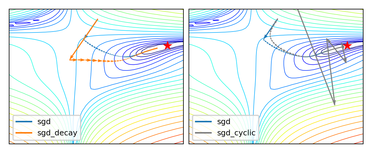
../_images/c32cd10a9f3fe5176b6f2b088b0a70be0434fd0f7f847fa254de09bde1eca29e.png

SGD with learning rate schedules#

Learning rate decay/annealing with decay rate $k$
- E.g. exponential ($\eta_{s+1} = \eta_{0} e^{-ks}$), inverse-time ($\eta_{s+1} = \frac{\eta_{0}}{1+ks}$),…
Cyclical learning rates
- Change from small to large: hopefully in ‘good’ region long enough before diverging
- Warm restarts: aggressive decay + reset to initial learning rate

../_images/04e6b15a8e1fc87478207003ef1099be531010ad770b764c1accb89d724a969d.png

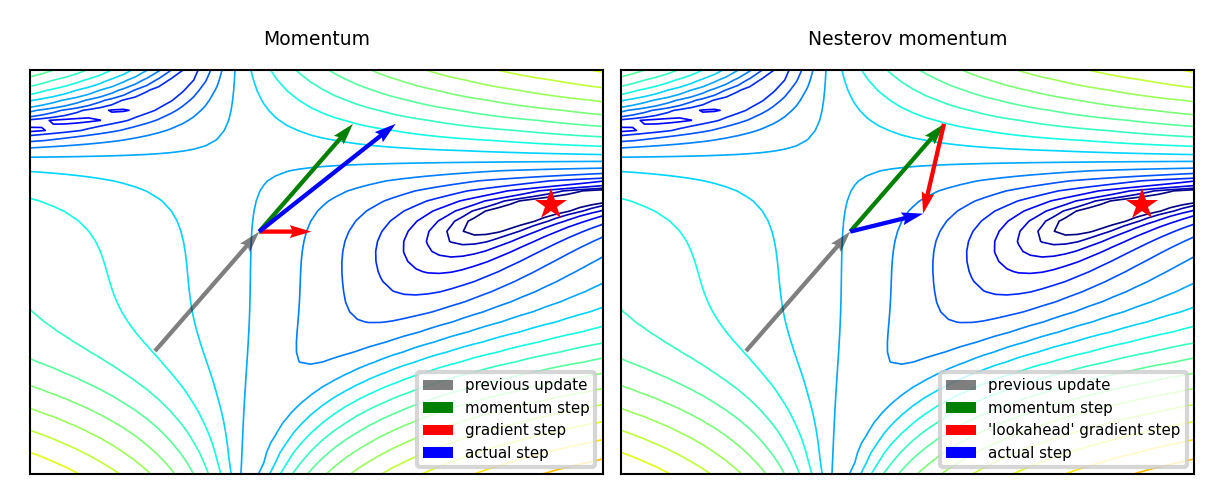
Momentum#

Imagine a ball rolling downhill: accumulates momentum, doesn’t exactly follow steepest descent
- Reduces oscillation, follows larger (consistent) gradient of the loss surface
Adds a velocity vector $\mathbf{v}$ with momentum $\gamma$ (e.g. 0.9, or increase from $\gamma=0.5$ to $\gamma=0.99$) $$\mathbf{w}_{(s+1)} = \mathbf{w}_{(s)} + \mathbf{v}_{(s)} \qquad \text{with} \qquad \color{blue}{\mathbf{v}_{(s)}} = \color{green}{\gamma \mathbf{v}_{(s-1)}} - \color{red}{\eta \nabla \mathcal{L}(\mathbf{w}_{(s)})}$$
Nesterov momentum: Look where momentum step would bring you, compute gradient there
- Responds faster (and reduces momentum) when the gradient changes $$\color{blue}{\mathbf{v}_{(s)}} = \color{green}{\gamma \mathbf{v}_{(s-1)}} - \color{red}{\eta \nabla \mathcal{L}(\mathbf{w}_{(s)} + \gamma \mathbf{v}_{(s-1)})}$$

../_images/e7432adc6200e9a2c7e89707e33266a5367d6387d037c223a613867899f0d646.png

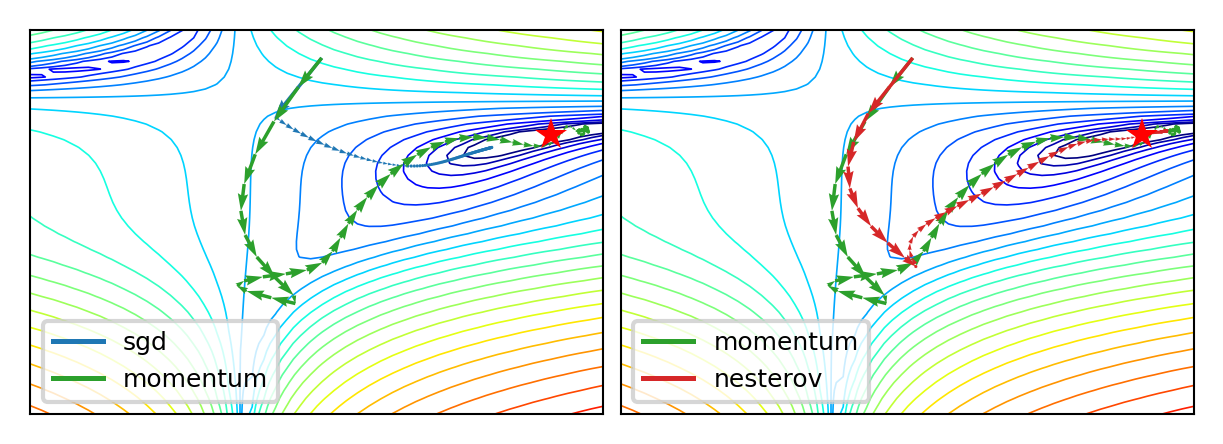
Momentum in practice#

../_images/248b8f48cea90e2e2cc5e461e732ab2d360974b986b850cceac323d3689bfa53.png

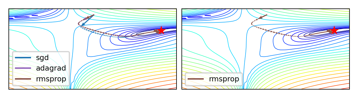
Adaptive gradients#

‘Correct’ the learning rate for each $w_i$ based on specific local conditions (layer depth, fan-in,…)
Adagrad: scale $\eta$ according to squared sum of previous gradients $G_{i,(s)} = \sum_{t=1}^s \nabla \mathcal{L}(w_{i,(t)})^2$
- Update rule for $w_i$. Usually $\epsilon=10^{-7}$ (avoids division by 0), $\eta=0.001$. $$w_{i,(s+1)} = w_{i,(s)} - \frac{\eta}{\sqrt{G_{i,(s)}+\epsilon}} \nabla \mathcal{L}(w_{i,(s)})$$
RMSProp: use moving average of squared gradients $m_{i,(s)} = \gamma m_{i,(s-1)} + (1-\gamma) \nabla \mathcal{L}(w_{i,(s)})^2$
- Avoids that gradients dwindle to 0 as $G_{i,(s)}$ grows. Usually $\gamma=0.9, \eta=0.001$ $$w_{i,(s+1)} = w_{i,(s)}- \frac{\eta}{\sqrt{m_{i,(s)}+\epsilon}} \nabla \mathcal{L}(w_{i,(s)})$$

../_images/c53cc403ce501754c9ae246462d4b9c390488d39974c6f6ff3ab3a16cc9cc48b.png

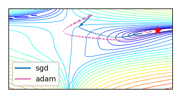
Adam (Adaptive moment estimation)#

Adam: RMSProp + momentum. Adds moving average for gradients as well ($\gamma_2$ = momentum):
- Adds a bias correction to avoid small initial gradients: $\hat{m}_{i,(s)} = \frac{m_{i,(s)}}{1-\gamma}$ and $\hat{g}_{i,(s)} = \frac{g_{i,(s)}}{1-\gamma_2}$ $$g_{i,(s)} = \gamma_2 g_{i,(s-1)} + (1-\gamma_2) \nabla \mathcal{L}(w_{i,(s)})$$w_{i,(s+1)} = w_{i,(s)}- \frac{\eta}{\sqrt{\hat{m}_{i,(s)}+\epsilon}} \hat{g}_{i,(s)}$$
Adamax: Idem, but use max() instead of moving average: $u_{i,(s)} = max(\gamma u_{i,(s-1)}, |\mathcal{L}(w_{i,(s)})|)$ $$w_{i,(s+1)} = w_{i,(s)}- \frac{\eta}{u_{i,(s)}} \hat{g}_{i,(s)}$$

../_images/5be02b6a7ead865f70a22ee9967e547df87d9511537ae9e0fff1687b1ebda853.png

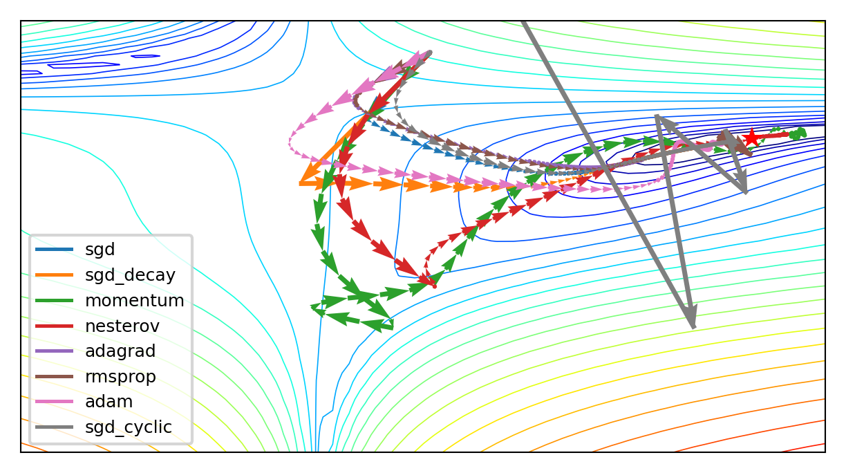
SGD Optimizer Zoo#

RMSProp often works well, but do try alternatives. For even more optimizers, see here.

../_images/be3aff8b685ccc51bd7f99bf7600e0adfdea55e0a2aaa536022d8c07300bd69f.png

Neural networks in practice#

There are many practical courses on training neural nets.
- E.g.: https://pytorch.org/tutorials/, fast.ai course
We’ll use PyTorch in these examples and the labs.
Focus on key design decisions, evaluation, and regularization
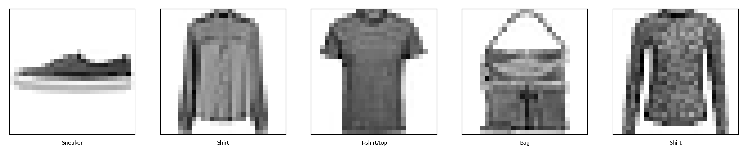
Running example: Fashion-MNIST
- 28x28 pixel images of 10 classes of fashion items

../_images/a8c28ac8664d72b67537a8dc07cbf7b62cd950aa1d8c815d77270ba37016a526.png

Preparing the data#

We’ll use feed-forward networks first, so we flatten the input data
Create train-test splits to evaluate the model later
Convert the data (numpy arrays) to PyTorch tensors

# Flatten images, create train-test split
X_flat = X.reshape(70000, 28 * 28)
X_train, X_test, y_train, y_test = train_test_split(X_flat, y, stratify=y)

# Convert numpy arrays to PyTorch tensors with correct types
X_train_tensor = torch.tensor(X_train, dtype=torch.float32)
y_train_tensor = torch.tensor(y_train, dtype=torch.long)
X_test_tensor = torch.tensor(X_test, dtype=torch.float32)
y_test_tensor = torch.tensor(y_test, dtype=torch.long)

Create data loaders to return data in batches

import torch
from torch.utils.data import DataLoader, TensorDataset

# Create PyTorch datasets
train_dataset = TensorDataset(X_train_tensor, y_train_tensor)
test_dataset = TensorDataset(X_test_tensor, y_test_tensor)

# Create DataLoaders
batch_size = 64
train_loader = DataLoader(train_dataset, batch_size=batch_size, shuffle=True)
test_loader = DataLoader(test_dataset, batch_size=batch_size, shuffle=False)

import torch
from sklearn.model_selection import train_test_split
from torch.utils.data import DataLoader, TensorDataset

# Flatten images, create train-test split
X_flat = X.reshape(70000, 28 * 28)
X_train, X_test, y_train, y_test = train_test_split(X_flat, y, stratify=y)

# Convert numpy arrays to PyTorch tensors with correct types
X_train_tensor = torch.tensor(X_train, dtype=torch.float32)
y_train_tensor = torch.tensor(y_train, dtype=torch.long)
X_test_tensor = torch.tensor(X_test, dtype=torch.float32)
y_test_tensor = torch.tensor(y_test, dtype=torch.long)


# Create PyTorch datasets
train_dataset = TensorDataset(X_train_tensor, y_train_tensor)
test_dataset = TensorDataset(X_test_tensor, y_test_tensor)

# Create DataLoaders
batch_size = 32
train_loader = DataLoader(train_dataset, batch_size=batch_size, num_workers=4, shuffle=True, pin_memory=False)
test_loader = DataLoader(test_dataset, batch_size=batch_size, num_workers=4, shuffle=False, pin_memory=False)

Building the network#

PyTorch has a Sequential and Functional API. We’ll use the Sequential API first.
Input layer: a flat vector of 28*28 = 784 nodes
- We’ll see how to properly deal with images later
Two dense (Linear) hidden layers: 512 nodes each, ReLU activation
Output layer: 10 nodes (for 10 classes)
- SoftMax not needed, it will be done in the loss function

import torch.nn as nn

model = nn.Sequential(
    nn.Linear(28 * 28, 512), # Layer 1: 28*28 inputs to 512 output nodes
    nn.ReLU(),
    nn.Linear(512, 512), # Layer 2: 512 inputs to 512 output nodes
    nn.ReLU(),
    nn.Linear(512, 10), # Layer 3: 512 inputs to output nodes
)

In the Functional API, the same network looks like this

import torch.nn.functional as F

class NeuralNetwork(nn.Module): # Class that defines your model
    def __init__(self):
        super(NeuralNetwork, self).__init__() # Components defined in __init__
        self.fc1 = nn.Linear(28 * 28, 512)    # Fully connected layers
        self.fc2 = nn.Linear(512, 512)
        self.fc3 = nn.Linear(512, 10)

    def forward(self, x):        # Forward pass and structure of the network
        x = F.relu(self.fc1(x))  # Layer 1: Input to FC1, then through ReLU
        x = F.relu(self.fc2(x))  # Layer 2: Then though FC2, then ReLU
        x = self.fc3(x)          # Layer 3: Then though FC3, then SoftMax
        return x                 # Return output

model = NeuralNetwork()

import torch.nn as nn
import torch.nn.functional as F

class NeuralNetwork(nn.Module): # Class that defines your model
    def __init__(self):
        super(NeuralNetwork, self).__init__() # Main components often defined in __init__
        self.fc1 = nn.Linear(28 * 28, 512)    # Fully connected layers
        self.fc2 = nn.Linear(512, 512)
        self.fc3 = nn.Linear(512, 10)

    def forward(self, x):                 # Forward pass and structure of the network
        x = F.relu(self.fc1(x))           # Layer 1: Input to FC1, then through ReLU
        x = F.relu(self.fc2(x))           # Layer 2: Then though FC2, then ReLU
        x = self.fc3(x)                   # Layer 3: Then though FC3, then SoftMax
        return x                          # Return output

model = NeuralNetwork()

Choosing loss, optimizer, metrics#

Loss function: Cross-entropy (log loss) for multi-class classification
Optimizer: Any of the optimizers we discussed before. RMSprop/Adam usually work well.
Metrics: To monitor performance during training and testing, e.g. accuracy

import torch.optim as optim
import torchmetrics

# Loss function with label smoothing. Also applies softmax internally
criterion = nn.CrossEntropyLoss(label_smoothing=0.01)

# Optimizer. Note that we pass the model parameters at creation time.
optimizer = optim.RMSprop(model.parameters(), lr=0.001, momentum=0.0)

# Accuracy metric
accuracy_metric = torchmetrics.Accuracy(task="multiclass", num_classes=10)

import torch.optim as optim
import torchmetrics

cross_entropy = nn.CrossEntropyLoss(label_smoothing=0.01)
optimizer = optim.RMSprop(model.parameters(), lr=0.001, momentum=0.0)
accuracy_metric = torchmetrics.Accuracy(task="multiclass", num_classes=10)

Training on GPU#

The device is where the training is done. It’s “cpu” by default.
The model, tensors, and metric must all be moved to the same device.

if torch.cuda.is_available():         # For CUDA based systems
    device = torch.device("cuda")
if torch.backends.mps.is_available(): # For MPS (M1-M4 Mac) based systems
    device = torch.device("mps")
print(f"Used device: {device}")

# Move models and metrics to `device`
model.to(device)                      
accuracy_metric = accuracy_metric.to(device)

# Move batches one at a time (GPUs have limited memory)
for X_batch, y_batch in train_loader:
    X_batch, y_batch = X_batch.to(device), y_batch.to(device)  

if torch.cuda.is_available():         # For CUDA based systems
    device = torch.device("cuda")
if torch.backends.mps.is_available(): # For MPS (M1-M4 Mac) based systems
    device = torch.device("mps")
print(f"Used device: {device}")

# Move everything to `device`
model.to(device)                      
accuracy_metric = accuracy_metric.to(device)
for X_batch, y_batch in train_loader:  
    X_batch, y_batch = X_batch.to(device), y_batch.to(device)  
    break

Used device: mps

Training loop#

In pure PyTorch, you have to write the training loop yourself (as well as any code to print out progress)

for epoch in range(10):
    for X_batch, y_batch in train_loader:
        X_batch, y_batch = X_batch.to(device), y_batch.to(device) # to GPU

        # Forward pass + loss calculation
        outputs = model(X_batch)
        loss = cross_entropy(outputs, y_batch)

        # Backward pass
        optimizer.zero_grad() # Reset gradients (otherwise they accumulate)
        loss.backward()       # Backprop. Computes all gradients
        optimizer.step()      # Uses gradients to update weigths

num_epochs = 5
for epoch in range(5):
    total_loss, correct, total = 0, 0, 0

    for X_batch, y_batch in train_loader:
        X_batch, y_batch = X_batch.to(device), y_batch.to(device) # to GPU

        # Forward pass + loss calculation
        outputs = model(X_batch)
        loss = cross_entropy(outputs, y_batch)

        # Backward pass: zero gradients, do backprop, do optimizer step
        optimizer.zero_grad()
        loss.backward()
        optimizer.step()

        # Compute training metrics
        total_loss += loss.item()
        correct += accuracy_metric(outputs, y_batch).item() * y_batch.size(0)
        total += y_batch.size(0)

    # Compute epoch metrics
    avg_loss = total_loss / len(train_loader)
    avg_acc = correct / total
    print(f"Epoch [{epoch+1}/{num_epochs}], Loss: {avg_loss:.4f}, Accuracy: {avg_acc:.4f}")

Epoch [1/5], Loss: 2.3524, Accuracy: 0.7495
Epoch [2/5], Loss: 0.5531, Accuracy: 0.8259
Epoch [3/5], Loss: 0.5102, Accuracy: 0.8408
Epoch [4/5], Loss: 0.4897, Accuracy: 0.8493
Epoch [5/5], Loss: 0.4758, Accuracy: 0.8550

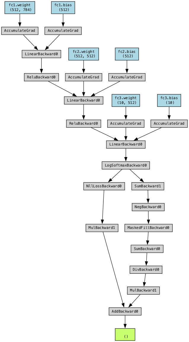
`loss.backward()`#

Every time you perform a forward pass, PyTorch dynamically constructs a computational graph
- This graph tracks tensors and operations involved in computing gradients (see next slide)
The loss returned is a tensor, and every tensor is part of the computational graph
When you call .backward() on loss, PyTorch traverses this graph in reverse to compute all gradients
- This process is called automatic differentiation
- Stores intermediate values so no gradient component is calculated twice
When backward() completes, the computational graph is discarded by default to free memory

Computational graph for our model (Loss in green, weights/biases in blue)

from torchviz import make_dot
from IPython.display import Image

toy_X = X_train_tensor[0].to(device)
toy_y = y_train_tensor[0].to(device)
toy_out = model(toy_X)
loss = cross_entropy(toy_out, toy_y)

graph = make_dot(loss, params=dict(model.named_parameters()))
graph.render("computational_graph", format="png", view=True)
Image("computational_graph.png")

../_images/4bca4d09b7b1a585b3c6417f53ddaf6f0d9b04e7ab7656415d4c9830a9971881.png

In PyTorch Lightning#

A high-level framework built on PyTorch that simplifies deep learning model training
Same code, but extend pl.LightingModule instead of nn.Module
Has a number of predefined functions. For instance:

class NeuralNetwork(pl.LightningModule):
    def __init__(self):
        pass # Initialize model
    
    def forward(self, x): 
        pass # Forward pass, return output tensor
    
    def configure_optimizers(self):
        pass # Configure optimizer (e.g. Adam)
    
    def training_step(self, batch, batch_idx):
        pass # Return loss tensor
    
    def validation_step(self, batch, batch_idx):
        pass # Return loss tensor
        
    def test_step(self, batch, batch_idx):
        pass # Return loss tensor

Our entire example now becomes:

import pytorch_lightning as pl

class NeuralNetwork(pl.LightningModule):
    def __init__(self):
        super(LitNeuralNetwork, self).__init__()
        self.fc1 = nn.Linear(28 * 28, 512)
        self.fc2 = nn.Linear(512, 512)
        self.fc3 = nn.Linear(512, 10)
        self.criterion = nn.CrossEntropyLoss(label_smoothing=0.01)
        self.accuracy = torchmetrics.Accuracy(task="multiclass", num_classes=10)

    def forward(self, x):
        x = F.relu(self.fc1(x))
        x = F.relu(self.fc2(x))
        return self.fc3(x)

    def training_step(self, batch, batch_idx):
        X_batch, y_batch = batch
        outputs = self(X_batch)
        return self.criterion(outputs, y_batch)

    def configure_optimizers(self):
        return optim.RMSprop(self.parameters(), lr=0.001, momentum=0.0)

model = NeuralNetwork()    

import pytorch_lightning as pl

class NeuralNetwork(pl.LightningModule):
    def __init__(self):
        super(NeuralNetwork, self).__init__()
        self.fc1 = nn.Linear(28 * 28, 512)
        self.fc2 = nn.Linear(512, 512)
        self.fc3 = nn.Linear(512, 10)
        self.criterion = nn.CrossEntropyLoss(label_smoothing=0.01)
        self.accuracy = torchmetrics.Accuracy(task="multiclass", num_classes=10)

    def forward(self, x):
        x = x.view(x.size(0), -1)  # Flatten the image
        x = F.relu(self.fc1(x))
        x = F.relu(self.fc2(x))
        return self.fc3(x)

    def training_step(self, batch, batch_idx):
        X_batch, y_batch = batch
        outputs = self(X_batch)                 # Logits (raw outputs)
        loss = self.criterion(outputs, y_batch) # Loss
        preds = torch.argmax(outputs, dim=1)    # Predictions
        acc = self.accuracy(preds, y_batch)
        self.log("train_loss", loss, sync_dist=True)
        self.log("train_acc", acc, sync_dist=True)
        return loss
    
    def validation_step(self, batch, batch_idx):
        X_batch, y_batch = batch
        outputs = self(X_batch)
        loss = self.criterion(outputs, y_batch)
        preds = torch.argmax(outputs, dim=1)
        acc = self.accuracy(preds, y_batch)
        self.log("val_loss", loss, sync_dist=True, on_epoch=True)
        self.log("val_acc", acc, sync_dist=True, on_epoch=True)
        return loss
    
    def on_train_epoch_end(self):
        avg_loss = self.trainer.callback_metrics["train_loss"].item()
        avg_acc = self.trainer.callback_metrics["train_acc"].item()
        print(f"Epoch {self.trainer.current_epoch+1}: Loss = {avg_loss:.4f}, Accuracy = {avg_acc:.4f}")

    def configure_optimizers(self):
        return optim.RMSprop(self.parameters(), lr=0.001, momentum=0.0)

model = NeuralNetwork()   

We can also get a nice model summary

Lots of parameters (weights and biases) to learn!
- hidden layer 1 : (28 * 28 + 1) * 512 = 401920
- hidden layer 2 : (512 + 1) * 512 = 262656
- output layer: (512 + 1) * 10 = 5130

ModelSummary(pl_model, max_depth=2)

  | Name      | Type               | Params | Mode 
---------------------------------------------------------
| fc1       | Linear             | 401 K  | train
| fc2       | Linear             | 262 K  | train
| fc3       | Linear             | 5.1 K  | train
| criterion | CrossEntropyLoss   | 0      | train
| accuracy  | MulticlassAccuracy | 0      | train
---------------------------------------------------------
K     Trainable params
       Non-trainable params
K     Total params
679     Total estimated model params size (MB)
       Modules in train mode
       Modules in eval mode

Training#

To log results while training, we can extend the training methods:

def training_step(self, batch, batch_idx):
    X_batch, y_batch = batch
    outputs = self(X_batch)                 # Logits (raw outputs)
    loss = self.criterion(outputs, y_batch) # Loss
    preds = torch.argmax(outputs, dim=1)    # Predictions
    acc = self.accuracy(preds, y_batch)     # Metric
    self.log("train_loss", loss)            # self.log is the default
    self.log("train_acc", acc)              # TensorBoard logger
    return loss

def on_train_epoch_end(self): # Runs at the end of every epoch
    avg_loss = self.trainer.callback_metrics["train_loss"].item()
    avg_acc = self.trainer.callback_metrics["train_acc"].item()
    print(f"Epoch {self.trainer.current_epoch}: Loss = {avg_loss:.4f}, Train accuracy = {avg_acc:.4f}")

We also need to implement the validation steps if we want validation scores

Identical to training_step except for the logging

def validation_step(self, batch, batch_idx):
    X_batch, y_batch = batch
    outputs = self(X_batch)
    loss = self.criterion(outputs, y_batch)
    preds = torch.argmax(outputs, dim=1)
    acc = self.accuracy(preds, y_batch)
    self.log("val_loss", loss, on_epoch=True)
    self.log("val_acc", acc, on_epoch=True)
    return loss

Lightning Trainer#

For training, we can now create a trainer and fit it. This will also automatically move everything to GPU.

trainer = pl.Trainer(max_epochs=3, accelerator="gpu") # Or 'cpu'
trainer.fit(model, train_loader)

import logging # Cleaner output
logging.getLogger("pytorch_lightning").setLevel(logging.ERROR)

accelerator = "cpu"
if torch.backends.mps.is_available():
    accelerator = "mps"
if torch.cuda.is_available():
    accelerator = "gpu"

trainer = pl.Trainer(max_epochs=3, accelerator=accelerator)
trainer.fit(model, train_loader)

Epoch 1: Loss = 0.6928, Accuracy = 0.8000
Epoch 2: Loss = 0.3986, Accuracy = 0.9000
Epoch 3: Loss = 0.3572, Accuracy = 0.9000

Choosing training hyperparameters#

Number of epochs: enough to allow convergence
- Too much: model starts overfitting (or levels off and just wastes time)
Batch size: small batches (e.g. 32, 64,… samples) often preferred
- ‘Noisy’ training data makes overfitting less likely
  - Large batches generalize less well (‘generalization gap’)
- Requires less memory (especially in GPUs)
- Large batches do speed up training, may converge in fewer epochs
Batch size interacts with learning rate
- Instead of shrinking the learning rate you can increase batch size

# Same model, more silent
class NeuralNetwork(pl.LightningModule):
    def __init__(self):
        super(NeuralNetwork, self).__init__()
        self.fc1 = nn.Linear(28 * 28, 512)
        self.fc2 = nn.Linear(512, 512)
        self.fc3 = nn.Linear(512, 10)
        self.criterion = nn.CrossEntropyLoss(label_smoothing=0.01)
        self.accuracy = torchmetrics.Accuracy(task="multiclass", num_classes=10)

    def forward(self, x):
        x = x.view(x.size(0), -1)  # Flatten the image
        x = F.relu(self.fc1(x))
        x = F.relu(self.fc2(x))
        return self.fc3(x)

    def training_step(self, batch, batch_idx):
        X_batch, y_batch = batch
        outputs = self(X_batch)                 # Logits (raw outputs)
        loss = self.criterion(outputs, y_batch) # Loss
        preds = torch.argmax(outputs, dim=1)    # Predictions
        acc = self.accuracy(preds, y_batch)
        self.log("train_loss", loss, sync_dist=True)
        self.log("train_acc", acc, sync_dist=True)
        return loss
    
    def validation_step(self, batch, batch_idx):
        X_batch, y_batch = batch
        outputs = self(X_batch)
        loss = self.criterion(outputs, y_batch)
        preds = torch.argmax(outputs, dim=1)
        acc = self.accuracy(preds, y_batch)
        self.log("val_loss", loss, sync_dist=True, on_epoch=True)
        self.log("val_acc", acc, sync_dist=True, on_epoch=True)
        return loss
    
    def on_train_epoch_end(self):
        avg_loss = self.trainer.callback_metrics["train_loss"].item()
        avg_acc = self.trainer.callback_metrics["train_acc"].item()
        
    def on_validation_epoch_end(self):
        avg_loss = self.trainer.callback_metrics["val_loss"].item()
        avg_acc = self.trainer.callback_metrics["val_acc"].item()

    def configure_optimizers(self):
        return optim.RMSprop(self.parameters(), lr=0.001, momentum=0.0)

model = NeuralNetwork() 

from pytorch_lightning.callbacks import Callback
from IPython.display import clear_output

# First try. Not very efficient yet.
class TrainingBatchPlotCallback(Callback):
    def __init__(self, update_interval=100, smoothing=100):
        """
        Callback to plot training and validation progress.

        Args:
            update_interval (int): Number of batches between updates.
            smoothing (int): Window size for moving average.
        """
        super().__init__()
        self.update_interval = update_interval
        self.smoothing = smoothing
        self.losses = []
        self.acc = []
        self.val_losses = []
        self.val_acc = []
        self.val_x_positions = []  # Store x positions for validation scores
        self.max_acc = 0
        self.global_step = 0  # Tracks processed training batches
        self.epoch_count = 0  # Tracks processed epochs
        self.steps_per_epoch = 0  # Updated dynamically to track num_batches per epoch

    def moving_average(self, values, window):
        """Computes a simple moving average for smoothing."""
        if len(values) < window:
            return np.convolve(values, np.ones(len(values)) / len(values), mode="valid")
        return np.convolve(values, np.ones(window) / window, mode="valid")

    def on_train_batch_end(self, trainer, pl_module, outputs, batch, batch_idx):
        """Updates training loss and accuracy every `update_interval` batches."""
        self.global_step += 1
        logs = trainer.callback_metrics

        # Store training loss and accuracy
        if "train_loss" in logs:
            self.losses.append(logs["train_loss"].item())
        if "train_acc" in logs:
            self.acc.append(logs["train_acc"].item())

        # Update plot every `update_interval` training batches
        if self.global_step % self.update_interval == 0:
            self.plot_progress()

    def on_validation_epoch_end(self, trainer, pl_module):
        """Updates validation loss and accuracy at the end of each epoch, scaling x-axis correctly."""
        logs = trainer.callback_metrics
        self.epoch_count += 1
        if self.steps_per_epoch == 0:
            self.steps_per_epoch = self.global_step

        self.val_x_positions.append(self.global_step)

        # Retrieve validation metrics from trainer
        if "val_loss" in logs:
            self.val_losses.append(logs["val_loss"].item())
        if "val_acc" in logs:
            val_acc = logs["val_acc"].item()
            self.val_acc.append(val_acc)
            self.max_acc = max(self.max_acc, val_acc)
            
    def on_train_end(self, trainer, pl_module):
        """Ensures the final validation curve is plotted after the last epoch."""
        self.plot_progress()
            
    def plot_progress(self):
        """Plots training and validation metrics with moving averages."""
        clear_output(wait=True)
        steps = np.arange(1, len(self.losses) + 1)

        plt.figure(figsize=(8, 4))
        plt.ylim(0, 1)  # Constrain y-axis between 0 and 1

        # Training curves
        plt.plot(steps / self.steps_per_epoch, self.losses, lw=0.2, alpha=0.3, c="b", linestyle="-")
        plt.plot(steps / self.steps_per_epoch, self.acc, lw=0.2, alpha=0.3, c="r", linestyle="-")

        # Moving average (thicker line)
        if len(self.losses) >= self.smoothing:
            plt.plot(steps[self.smoothing - 1:] / self.steps_per_epoch, self.moving_average(self.losses, self.smoothing),
                     lw=1, c="b", linestyle="-", label="Train Loss")
        if len(self.acc) >= self.smoothing:
            plt.plot(steps[self.smoothing - 1:] / self.steps_per_epoch, self.moving_average(self.acc, self.smoothing),
                     lw=1, c="r", linestyle="-", label="Train Acc")

        # Validation curves (scaled to correct x-positions)
        if self.val_losses:
            plt.plot(np.array(self.val_x_positions) / self.steps_per_epoch, self.val_losses, c="b", linestyle=":", label="Val Loss", lw=2)
        if self.val_acc:
            plt.plot(np.array(self.val_x_positions) / self.steps_per_epoch, self.val_acc, c="r", linestyle=":", label="Val Acc", lw=2)

        plt.xlabel("Epochs", fontsize=12)
        plt.ylabel("Loss/Accuracy", fontsize=12)
        plt.title(f"Training Progress (Step {self.global_step}, Epoch {self.epoch_count}, Max Val Acc {self.max_acc:.4f})", fontsize=12)
        plt.xticks(fontsize=10)
        plt.yticks(fontsize=10)
        plt.legend(fontsize=10)
        plt.show()

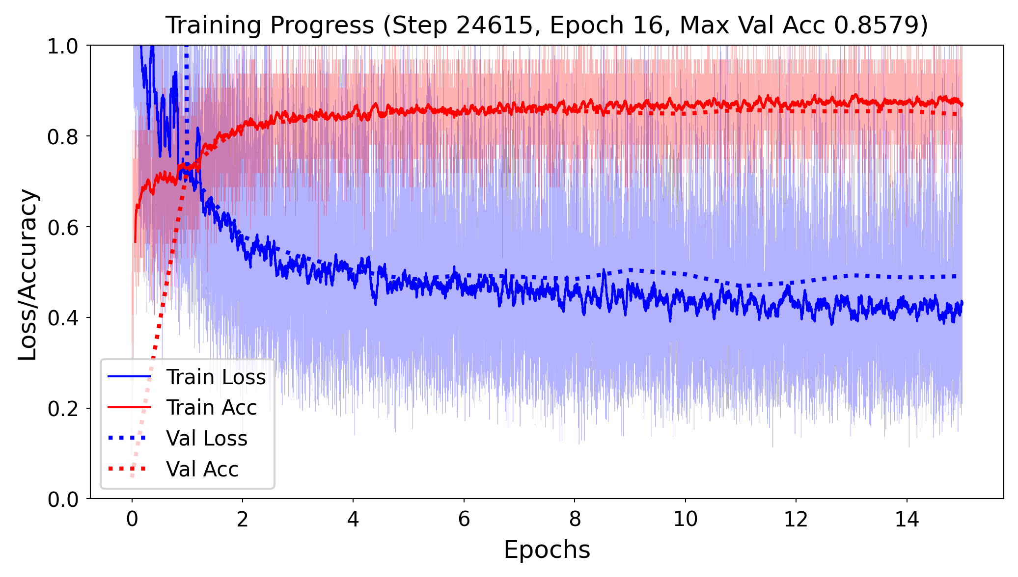
Model selection#

Train the neural net and track the loss after every iteration on a validation set
- You can add a callback to the fit version to get info on every epoch
Best model after a few epochs, then starts overfitting

trainer = pl.Trainer(
    max_epochs=15,
    enable_progress_bar=False,
    accelerator=accelerator,
    callbacks=[TrainingBatchPlotCallback()] # Attach the callback
)
trainer.fit(model, train_loader, test_loader)

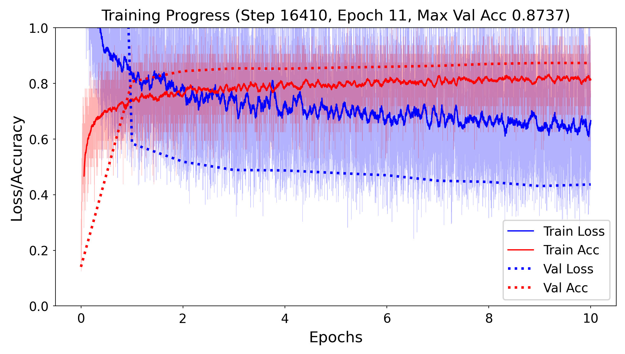
../_images/663540e274d5504b79dfc5ade3d5ee5ebe8faccebd81346356d8f46d2fdddc8f.png

Early stopping#

Stop training when the validation loss (or validation accuracy) no longer improves
Loss can be bumpy: use a moving average or wait for $k$ steps without improvement

# Define early stopping callback
early_stopping = EarlyStopping(
    monitor="val_loss", mode="min", # minimize validation loss
    patience=3)                     # Number of epochs with no improvement before stopping
          
# Update the Trainer to include early stopping as a callback
trainer = pl.Trainer(
    max_epochs=10, accelerator=accelerator,
    callbacks=[TrainingPlotCallback(), early_stopping]  # Attach the callbacks
)

Regularization and memorization capacity#

The number of learnable parameters is called the model capacity
A model with more parameters has a higher memorization capacity
- Too high capacity causes overfitting, too low causes underfitting
- In the extreme, the training set can be ‘memorized’ in the weights
Smaller models are forced it to learn a compressed representation that generalizes better
- Find the sweet spot: e.g. start with few parameters, increase until overfitting stars.
Example: 256 nodes in first layer, 32 nodes in second layer, similar performance
- Avoid bottlenecks: layers so small that information is lost

self.fc1 = nn.Linear(28 * 28, 256)
self.fc2 = nn.Linear(256, 32)
self.fc3 = nn.Linear(32, 10)

Weight regularization (weight decay)#

We can also add weight regularization to our loss function (or invent your own)

L1 regularization: leads to sparse networks with many weights that are 0
L2 regularization: leads to many very small weights

def training_step(self, batch, batch_idx):
    X_batch, y_batch = batch
    outputs = self(X_batch)                 
    loss = self.criterion(outputs, y_batch)
    l1_lambda = 1e-5 # L1 Regularization
    l1_loss = sum(p.abs().sum() for p in self.parameters())
    l2_lambda = 1e-4 # L2 Regularization
    l2_loss = sum((p ** 2).sum() for p in self.parameters())
    return loss + l2_lambda * l2_loss  # Using L2 only

Alternative: set weight_decay in the optimizer (only for L2 loss)

def configure_optimizers(self):
    return optim.RMSprop(self.parameters(), lr=0.001, momentum=0.0, weight_decay=1e-4)

Dropout#

Every iteration, randomly set a number of activations $a_i$ to 0
Dropout rate : fraction of the outputs that are zeroed-out (e.g. 0.1 - 0.5)
- Use higher dropout rates for deeper networks
Use higher dropout in early layers, lower dropout later
- Early layers are usually larger, deeper layers need stability
Idea: break up accidental non-significant learned patterns
At test time, nothing is dropped out, but the output values are scaled down by the dropout rate
- Balances out that more units are active than during training

../_images/42f3c29683ed37223f2b024ff3d1c6824d5d7e483c276a76483c1465f6693acd.png

Dropout layers#

Dropout is usually implemented as a special layer

def __init__(self):
    super(NeuralNetwork, self).__init__()
    self.fc1 = nn.Linear(28 * 28, 512)
    self.dropout1 = nn.Dropout(p=0.2)  # 20% dropout
    self.fc2 = nn.Linear(512, 512)
    self.dropout2 = nn.Dropout(p=0.1)  # 10% dropout
    self.fc3 = nn.Linear(512, 10)

def forward(self, x):
    x = F.relu(self.fc1(x))
    x = self.dropout1(x)  # Apply dropout
    x = F.relu(self.fc2(x))
    x = self.dropout2(x)  # Apply dropout
    return self.fc3(x)

Batch Normalization#

We’ve seen that scaling the input is important, but what if layer activations become very large?
- Same problems, starting deeper in the network
Batch normalization: normalize the activations of the previous layer within each batch
- Within a batch, set the mean activation close to 0 and the standard deviation close to 1
  - Across badges, use exponential moving average of batch-wise mean and variance
- Allows deeper networks less prone to vanishing or exploding gradients

BatchNorm layers#

Batch normalization is also usually implemented as a special layer

def __init__(self):
    super(NeuralNetwork, self).__init__()
    self.fc1 = nn.Linear(28 * 28, 512)
    self.bn1 = nn.BatchNorm1d(512)  # Batch normalization after first layer
    self.fc2 = nn.Linear(512, 265)
    self.bn2 = nn.BatchNorm1d(265)  # Batch normalization after second layer
    self.fc3 = nn.Linear(265, 10)

def forward(self, x):
    x = x.view(x.size(0), -1)  # Flatten the image
    x = F.relu(self.bn1(self.fc1(x)))  # Apply batch norm after linear layer
    x = F.relu(self.bn2(self.fc2(x)))  # Apply batch norm after second layer
    return self.fc3(x)

New model#

class NeuralNetwork(pl.LightningModule):
    def __init__(self):
        super(NeuralNetwork, self).__init__()
        self.fc1 = nn.Linear(28 * 28, 265)
        self.bn1 = nn.BatchNorm1d(265)
        self.dropout1 = nn.Dropout(0.5)
        self.fc2 = nn.Linear(265, 64)
        self.bn2 = nn.BatchNorm1d(64)
        self.dropout2 = nn.Dropout(0.5)
        self.fc3 = nn.Linear(64, 32)
        self.bn3 = nn.BatchNorm1d(32)
        self.dropout3 = nn.Dropout(0.5)
        self.fc4 = nn.Linear(32, 10)
        self.criterion = nn.CrossEntropyLoss(label_smoothing=0.01)
        self.accuracy = torchmetrics.Accuracy(task="multiclass", num_classes=10)

    def forward(self, x):
        x = F.relu(self.bn1(self.fc1(x)))
        x = self.dropout1(x)
        x = F.relu(self.bn2(self.fc2(x)))
        x = self.dropout2(x)
        x = F.relu(self.bn3(self.fc3(x)))
        x = self.dropout3(x)
        x = self.fc4(x)
        return x

New model (Sequential API)#

model = nn.Sequential(
        nn.Linear(28 * 28, 265),
        nn.BatchNorm1d(265),
        nn.ReLU(),
        nn.Dropout(0.5),
        nn.Linear(265, 64),
        nn.BatchNorm1d(64),
        nn.ReLU(),
        nn.Dropout(0.5),
        nn.Linear(64, 32),
        nn.BatchNorm1d(32),
        nn.ReLU(),
        nn.Dropout(0.5),
        nn.Linear(32, 10))

Our model now performs better and is improving.

class NeuralNetwork(pl.LightningModule):
    def __init__(self):
        super(NeuralNetwork, self).__init__()
        self.fc1 = nn.Linear(28 * 28, 265)
        self.bn1 = nn.BatchNorm1d(265)
        self.dropout1 = nn.Dropout(0.5)
        self.fc2 = nn.Linear(265, 64)
        self.bn2 = nn.BatchNorm1d(64)
        self.dropout2 = nn.Dropout(0.5)
        self.fc3 = nn.Linear(64, 32)
        self.bn3 = nn.BatchNorm1d(32)
        self.dropout3 = nn.Dropout(0.5)
        self.fc4 = nn.Linear(32, 10)
        self.accuracy = torchmetrics.Accuracy(task="multiclass", num_classes=10)
        self.criterion = nn.CrossEntropyLoss(label_smoothing=0.01)

    def forward(self, x):
        x = F.relu(self.bn1(self.fc1(x)))
        x = self.dropout1(x)
        x = F.relu(self.bn2(self.fc2(x)))
        x = self.dropout2(x)
        x = F.relu(self.bn3(self.fc3(x)))
        x = self.dropout3(x)
        x = self.fc4(x)
        return x

    def training_step(self, batch, batch_idx):
        X_batch, y_batch = batch
        outputs = self(X_batch)                 # Logits (raw outputs)
        loss = self.criterion(outputs, y_batch) # Loss
        preds = torch.argmax(outputs, dim=1)    # Predictions
        acc = self.accuracy(preds, y_batch)
        self.log("train_loss", loss, sync_dist=True)
        self.log("train_acc", acc, sync_dist=True)
        return loss
    
    def validation_step(self, batch, batch_idx):
        X_batch, y_batch = batch
        outputs = self(X_batch)
        loss = self.criterion(outputs, y_batch)
        preds = torch.argmax(outputs, dim=1)
        acc = self.accuracy(preds, y_batch)
        self.log("val_loss", loss, sync_dist=True, on_epoch=True)
        self.log("val_acc", acc, sync_dist=True, on_epoch=True)
        return loss
    
    def on_train_epoch_end(self):
        avg_loss = self.trainer.callback_metrics["train_loss"].item()
        avg_acc = self.trainer.callback_metrics["train_acc"].item()
        
    def on_validation_epoch_end(self):
        avg_loss = self.trainer.callback_metrics["val_loss"].item()
        avg_acc = self.trainer.callback_metrics["val_acc"].item()

    def configure_optimizers(self):
        return optim.RMSprop(self.parameters(), lr=0.001, momentum=0.0)
    
model = NeuralNetwork() 

trainer = pl.Trainer(
    max_epochs=10,
    enable_progress_bar=False,
    accelerator=accelerator,
    callbacks=[TrainingBatchPlotCallback()] # Attach the callback
)
trainer.fit(model, train_loader, test_loader)

../_images/172f6478b7699cdb59f49378fea9e10cd922e7a9d6f3635d9fa43d55c0d05e07.png

Other logging tools#

There is a lot more tooling to help you build good models
E.g. TensorBoard is easy to integrate and offers a convenient dashboard

logger = pl.loggers.TensorBoardLogger("logs/", name="my_experiment")
trainer = pl.Trainer(max_epochs=2, logger=logger)
trainer.fit(lit_model, trainloader)

Summary#

Neural architectures
Training neural nets
- Forward pass: Tensor operations
- Backward pass: Backpropagation
Neural network design:
- Activation functions
- Weight initialization
- Optimizers
Neural networks in practice
Model selection
- Early stopping
- Memorization capacity and information bottleneck
- L1/L2 regularization
- Dropout
- Batch normalization

Lecture 6. Neural Networks

Contents

Lecture 6. Neural Networks#

Overview#

Architecture#

Basic Architecture#

More layers#

Why layers?#

Other architectures#

Training Neural Nets#

Mini-batch Stochastic Gradient Descent (recap)#

Forward pass#

Tensor operations#

Element-wise operations#

Backward pass (backpropagation)#

Example#

Backpropagation (2)#

Backpropagation (3)#

Summary#

Activation functions for hidden layers#

Effect of activation functions on the gradient#

ReLU vs Tanh#

Activation functions for output layer#

Weight initialization#

Weight initialization: transfer learning#

Optimizers#

SGD with learning rate schedules#

SGD with learning rate schedules#

Momentum#

Momentum in practice#

Adaptive gradients#

Adam (Adaptive moment estimation)#

SGD Optimizer Zoo#

Neural networks in practice#

Preparing the data#

Building the network#

Choosing loss, optimizer, metrics#

Training on GPU#

Training loop#

loss.backward()#

In PyTorch Lightning#

Training#

Lightning Trainer#

Choosing training hyperparameters#

Model selection#

Early stopping#

Regularization and memorization capacity#

Weight regularization (weight decay)#

Dropout#

Dropout layers#

Batch Normalization#

BatchNorm layers#

New model#

New model (Sequential API)#

Other logging tools#

Summary#

`loss.backward()`#