
Recap: Data preprocessing#
Basic data transformation techniques
Joaquin Vanschoren
Show code cell source
# Auto-setup when running on Google Colab
import os
if 'google.colab' in str(get_ipython()) and not os.path.exists('/content/master'):
    !git clone -q https://github.com/ML-course/master.git /content/master
    !pip --quiet install -r /content/master/requirements_colab.txt
    %cd master/notebooks

# Global imports and settings
%matplotlib inline
from preamble import *
interactive = True # Set to True for interactive plots
if interactive:
    fig_scale = 0.9
    plt.rcParams.update(print_config)
else: # For printing
    fig_scale = 0.35
    plt.rcParams.update(print_config)
Data transformations covered here#
Scaling and power transformations
Unsupervised feature selection ()
Feature engineering (e.g. binning, polynomial features,…)
Handling missing data
Handling imbalanced data
Dimensionality reduction (e.g. PCA)
Learned embeddings (e.g. for text)
Seek the best combinations of transformations and learning methods
Often done empirically, using cross-validation
Make sure that there is no data leakage during this process!
Scaling#
Use when different numeric features have different scales (different range of values)
Features with much higher values may overpower the others
Goal: bring them all within the same range
Different methods exist
Show code cell source
from sklearn.datasets import fetch_openml
from sklearn.preprocessing import LabelEncoder, MinMaxScaler, StandardScaler, RobustScaler, Normalizer, MaxAbsScaler
import ipywidgets as widgets
from ipywidgets import interact, interact_manual

# Iris dataset with some added noise
def noisy_iris():
    iris = fetch_openml("iris", return_X_y=True, as_frame=False)
    X, y = iris
    np.random.seed(0)
    noise = np.random.normal(0, 0.1, 150)
    for i in range(4):
        X[:, i] = X[:, i] + noise
    X[:, 0] = X[:, 0] + 3 # add more skew
    label_encoder = LabelEncoder().fit(y)
    y = label_encoder.transform(y)
    return X, y

scalers = [StandardScaler(), RobustScaler(), MinMaxScaler(), Normalizer(norm='l1'), MaxAbsScaler()]

@interact
def plot_scaling(scaler=scalers):
    X, y = noisy_iris()
    X = X[:,:2] # Use only first 2 features

    fig, axes = plt.subplots(nrows=1, ncols=2, figsize=(8*fig_scale, 3*fig_scale))
    axes[0].scatter(X[:, 0], X[:, 1], c=y, s=1*fig_scale, cmap="brg")
    axes[0].set_xlim(-15, 15)
    axes[0].set_ylim(-5, 5)
    axes[0].set_title("Original Data")
    axes[0].spines['left'].set_position('zero')
    axes[0].spines['bottom'].set_position('zero')

    X_ = scaler.fit_transform(X)
    axes[1].scatter(X_[:, 0], X_[:, 1], c=y, s=1*fig_scale, cmap="brg")
    axes[1].set_xlim(-2, 2)
    axes[1].set_ylim(-2, 2)
    axes[1].set_title(type(scaler).__name__)
    axes[1].set_xticks([-1,1])
    axes[1].set_yticks([-1,1])
    axes[1].spines['left'].set_position('center')
    axes[1].spines['bottom'].set_position('center')

    for ax in axes:
        ax.spines['right'].set_color('none')
        ax.spines['top'].set_color('none')
        ax.xaxis.set_ticks_position('bottom')
        ax.yaxis.set_ticks_position('left')
Show code cell source
if not interactive:
    plot_scaling(scalers[0])
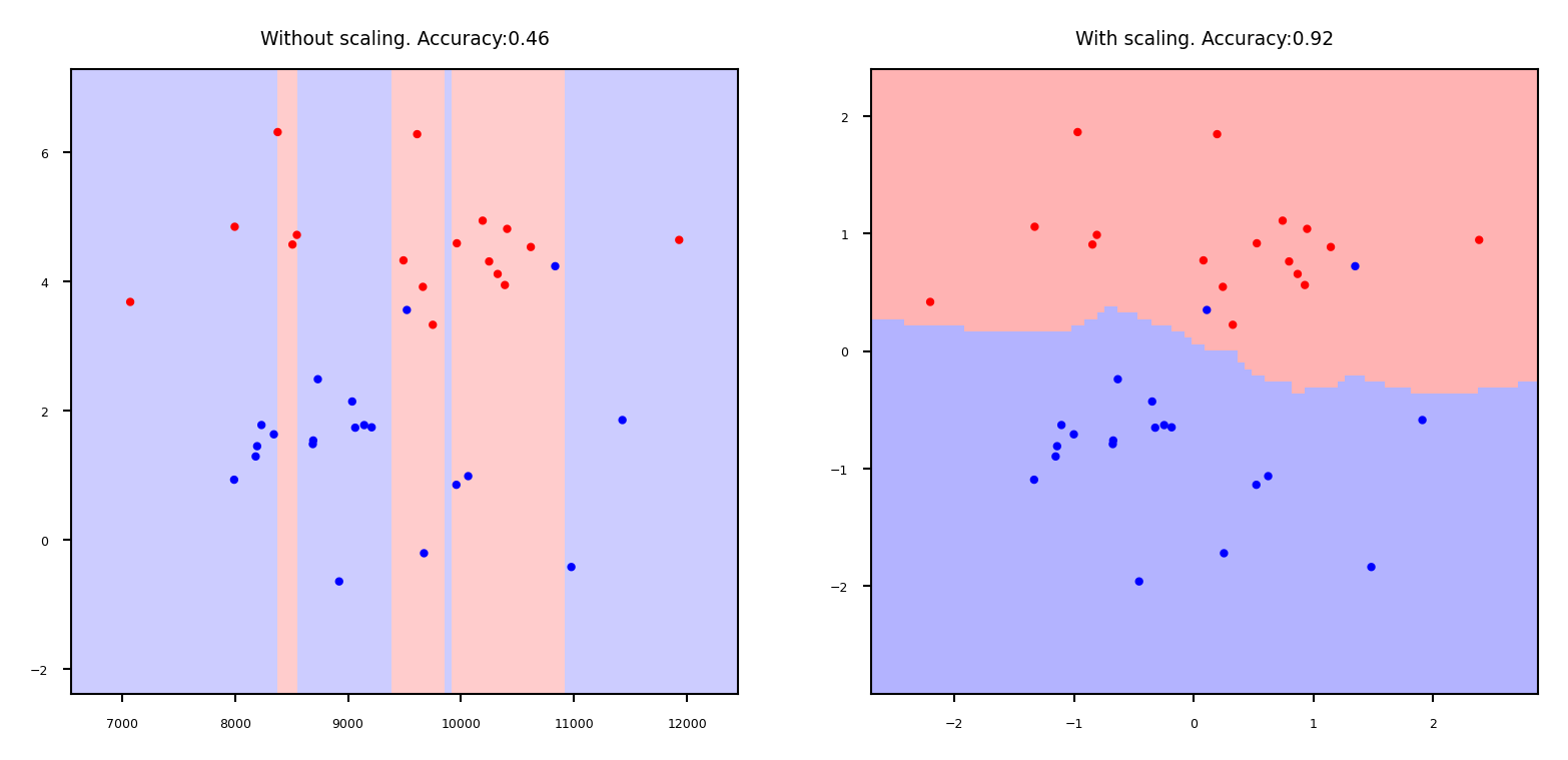
Why do we need scaling?#
KNN: Distances depend mainly on feature with larger values
SVMs: (kernelized) dot products are also based on distances
Linear model: Feature scale affects regularization
Weights have similar scales, more interpretable
Show code cell source
from sklearn.neighbors import KNeighborsClassifier
from sklearn.svm import SVC, LinearSVC
from sklearn.linear_model import LogisticRegression
from sklearn.datasets import make_blobs
from sklearn.model_selection import train_test_split
from sklearn.base import clone

# Example by Andreas Mueller, with some tweaks
def plot_2d_classification(classifier, X, fill=False, ax=None, eps=None, alpha=1):
    # multiclass
    if eps is None:
        eps = X.std(axis=0) / 2.
    else:
        eps = np.array([eps, eps])

    if ax is None:
        ax = plt.gca()

    x_min, x_max = X[:, 0].min() - eps[0], X[:, 0].max() + eps[0]
    y_min, y_max = X[:, 1].min() - eps[1], X[:, 1].max() + eps[1]
    # these should be 1000 but knn predict is unnecessarily slow
    xx = np.linspace(x_min, x_max, 100)
    yy = np.linspace(y_min, y_max, 100)

    X1, X2 = np.meshgrid(xx, yy)
    X_grid = np.c_[X1.ravel(), X2.ravel()]
    decision_values = classifier.predict(X_grid)
    ax.imshow(decision_values.reshape(X1.shape), extent=(x_min, x_max,
                                                       y_min, y_max),
            aspect='auto', origin='lower', alpha=alpha, cmap=plt.cm.bwr)

clfs = [KNeighborsClassifier(), SVC(), LinearSVC(), LogisticRegression(C=10)]

@interact
def plot_scaling_effect(classifier=clfs, show_test=[False,True]):
    X, y = make_blobs(centers=2, random_state=4, n_samples=50)
    X = X * np.array([1000, 1])
    y[7], y[27] = 0, 0
    X_train, X_test, y_train, y_test = train_test_split(X,y, stratify=y, random_state=1)

    clf2 = clone(classifier)
    clf_unscaled = classifier.fit(X_train, y_train)

    fig, axes = plt.subplots(1, 2, figsize=(7*fig_scale, 3*fig_scale))
    axes[0].scatter(X_train[:, 0], X_train[:, 1], c=y_train, cmap='bwr', label="train")
    axes[0].set_title("Without scaling. Accuracy:{:.2f}".format(clf_unscaled.score(X_test,y_test)))
    if show_test: # Hide test data for simplicity
        axes[0].scatter(X_test[:, 0], X_test[:, 1], c=y_test, marker='^', cmap='bwr', label="test")
        axes[0].legend()

    scaler = StandardScaler().fit(X_train)
    X_train_scaled = scaler.transform(X_train)
    X_test_scaled = scaler.transform(X_test)
    clf_scaled = clf2.fit(X_train_scaled, y_train)

    axes[1].scatter(X_train_scaled[:, 0], X_train_scaled[:, 1], c=y_train, cmap='bwr', label="train")
    axes[1].set_title("With scaling. Accuracy:{:.2f}".format(clf_scaled.score(X_test_scaled,y_test)))
    if show_test: # Hide test data for simplicity
        axes[1].scatter(X_test_scaled[:, 0], X_test_scaled[:, 1], c=y_test, marker='^', cmap='bwr', label="test")
        axes[1].legend()

    plot_2d_classification(clf_unscaled, X, ax=axes[0], alpha=.2)
    plot_2d_classification(clf_scaled, scaler.transform(X), ax=axes[1], alpha=.3)
Show code cell source
if not interactive:
    plot_scaling_effect(classifier=clfs[0], show_test=False)
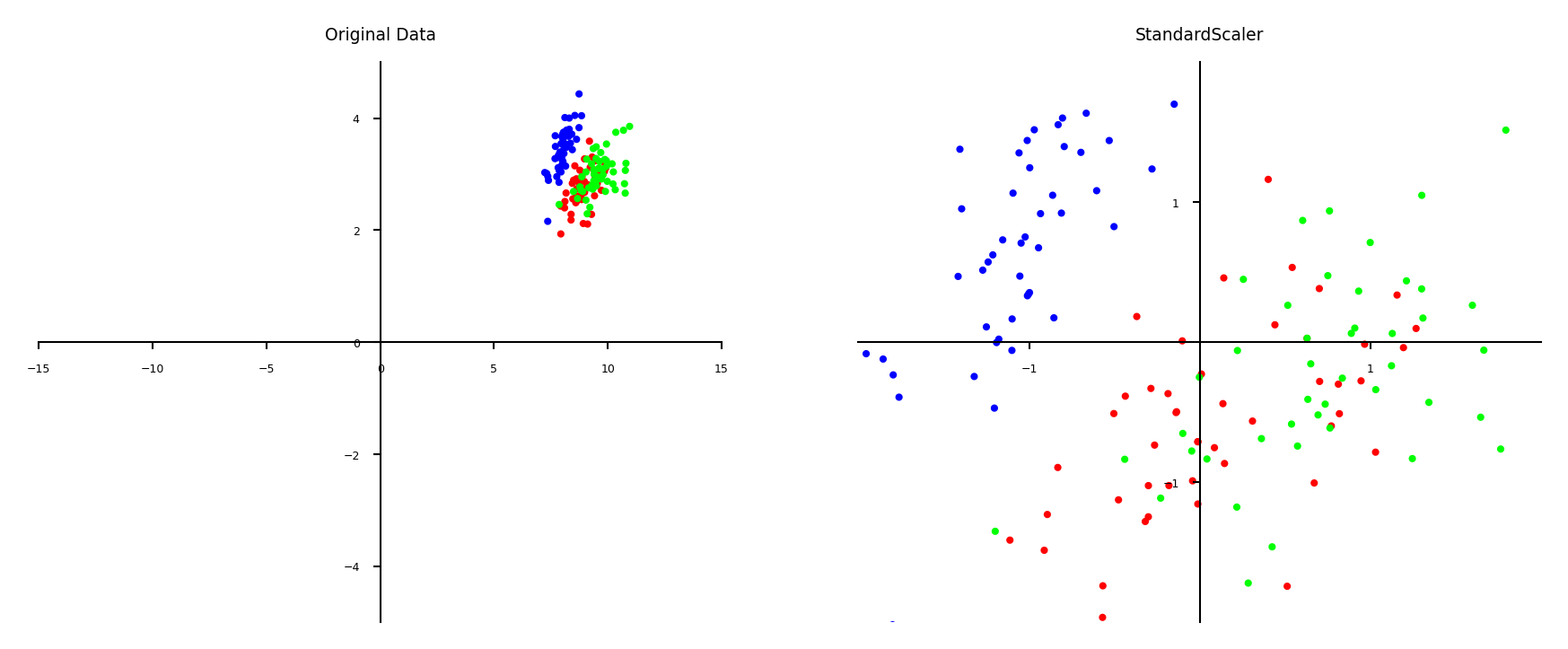
Standard scaling (standardization)#
Generally most useful, assumes data is more or less normally distributed
Per feature, subtract the mean value \(\mu\), scale by standard deviation \(\sigma\)
New feature has \(\mu=0\) and \(\sigma=1\), values can still be arbitrarily large $\(\mathbf{x}_{new} = \frac{\mathbf{x} - \mu}{\sigma}\)$
Show code cell source
plot_scaling(scaler=StandardScaler())
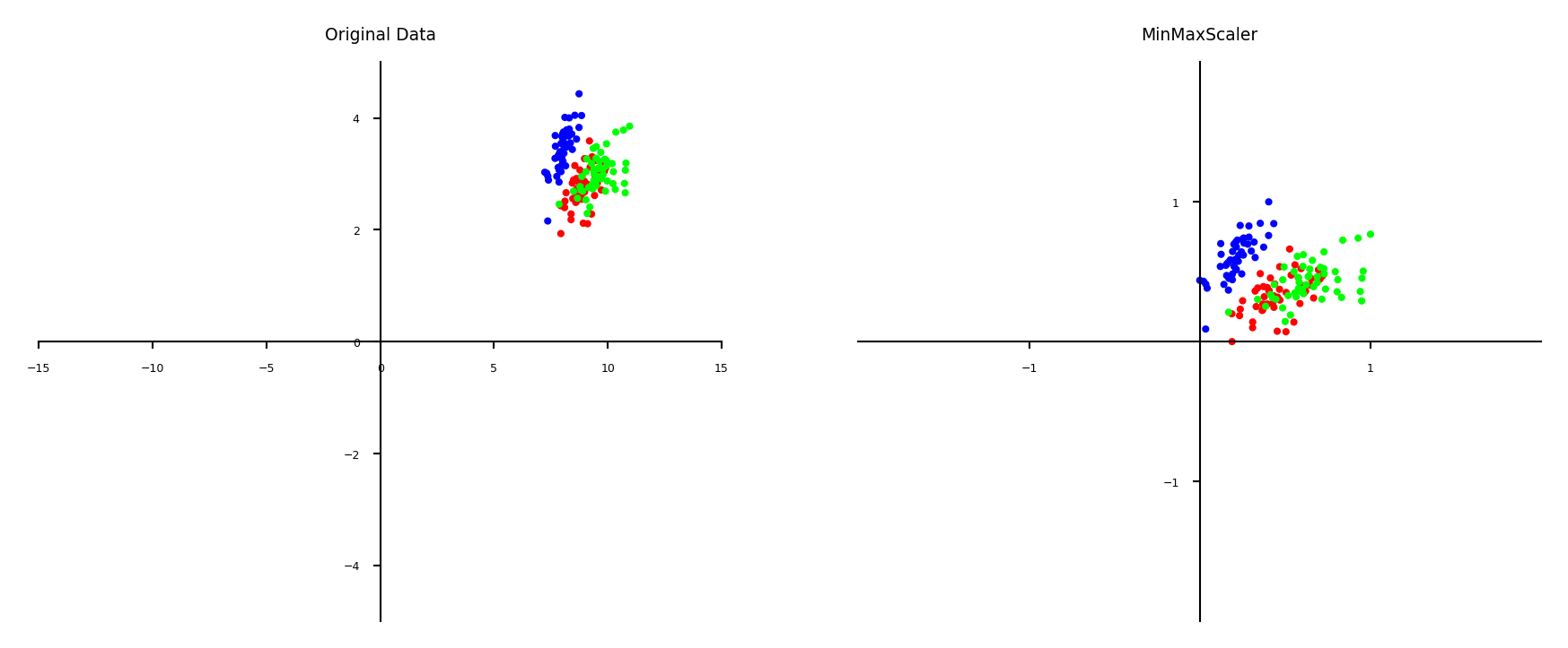
Min-max scaling#
Scales all features between a given \(min\) and \(max\) value (e.g. 0 and 1)
Makes sense if min/max values have meaning in your data
Sensitive to outliers
Show code cell source
plot_scaling(scaler=MinMaxScaler(feature_range=(0, 1)))
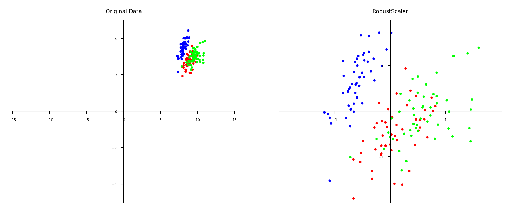
Robust scaling#
Subtracts the median, scales between quantiles \(q_{25}\) and \(q_{75}\)
New feature has median 0, \(q_{25}=-1\) and \(q_{75}=1\)
Similar to standard scaler, but ignores outliers
Show code cell source
plot_scaling(scaler=RobustScaler())
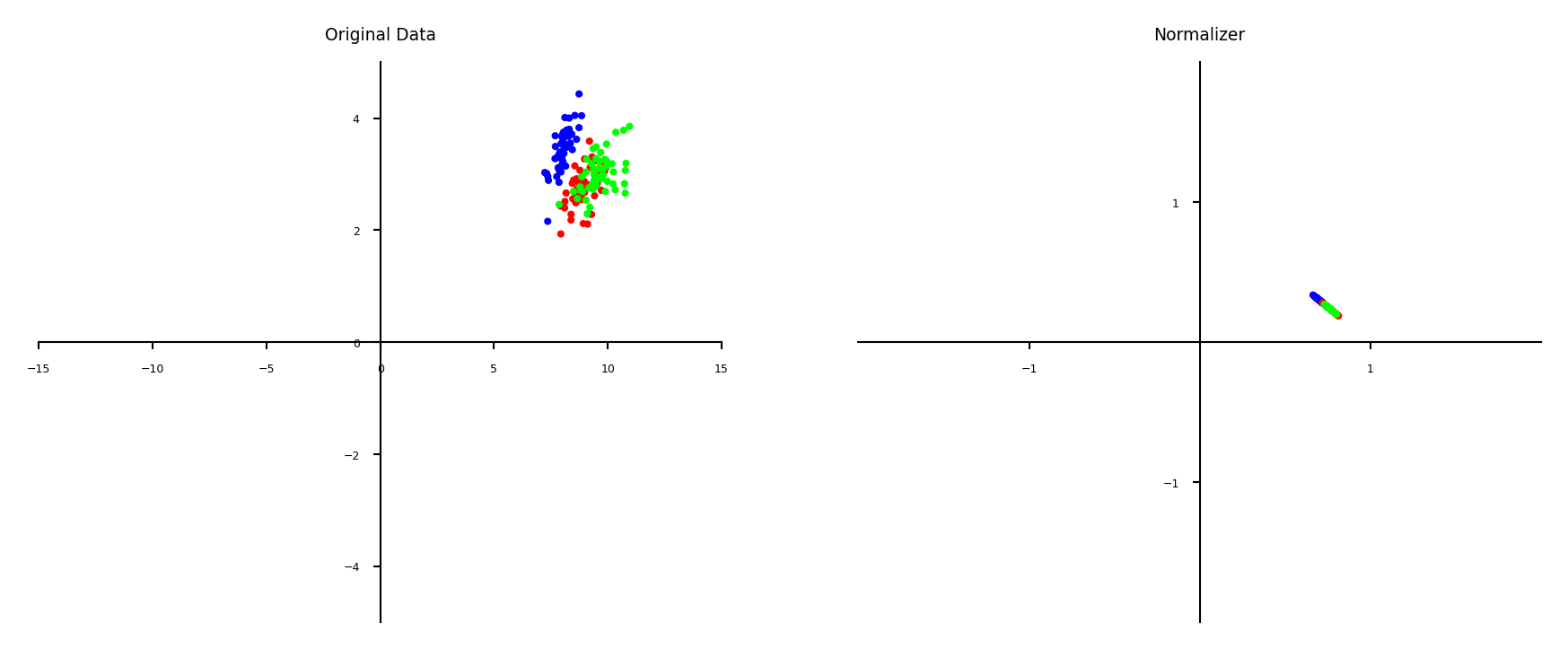
Normalization#
Makes sure that feature values of each point (each row) sum up to 1 (L1 norm)
Useful for count data (e.g. word counts in documents)
Can also be used with L2 norm (sum of squares is 1)
Useful when computing distances in high dimensions
Normalized Euclidean distance is equivalent to cosine similarity
Show code cell source
plot_scaling(scaler=Normalizer(norm='l1'))
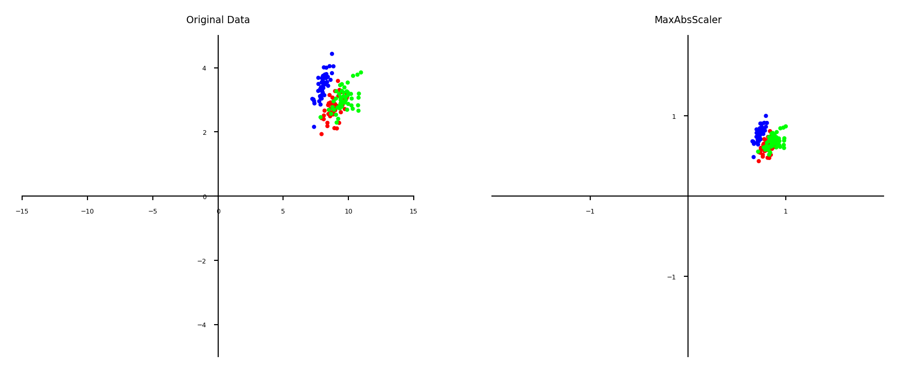
Maximum Absolute scaler#
For sparse data (many features, but few are non-zero)
Maintain sparseness (efficient storage)
Scales all values so that maximum absolute value is 1
Similar to Min-Max scaling without changing 0 values
Show code cell source
plot_scaling(scaler=MaxAbsScaler())
Automatic Feature Selection#
It can be a good idea to reduce the number of features to only the most useful ones
Simpler models that generalize better (less overfitting)
Curse of dimensionality (e.g. kNN)
Even models such as RandomForest can benefit from this
Sometimes it is one of the main methods to improve models (e.g. gene expression data)
Faster prediction and training
Training time can be quadratic (or cubic) in number of features
Easier data collection, smaller models (less storage)
More interpretable models: fewer features to look at
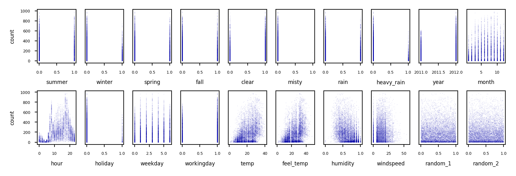
Example: bike sharing#
The Bike Sharing Demand dataset shows the amount of bikes rented in Washington DC
Some features are clearly more informative than others (e.g. temp, hour)
Some are correlated (e.g. temp and feel_temp)
We add two random features at the end
Show code cell source
from sklearn.datasets import fetch_openml
from sklearn.preprocessing import OneHotEncoder
from sklearn.compose import ColumnTransformer

# Get bike sharing data from OpenML
bikes = fetch_openml(data_id=42713, as_frame=True)
X_bike_cat, y_bike = bikes.data, bikes.target

# Optional: take half of the data to speed up processing
X_bike_cat = X_bike_cat.sample(frac=0.5, random_state=1)
y_bike = y_bike.sample(frac=0.5, random_state=1)

# One-hot encode the categorical features
encoder = OneHotEncoder(dtype=int)
preprocessor = ColumnTransformer(transformers=[('cat', encoder, [0,7])], remainder='passthrough')
X_bike = preprocessor.fit_transform(X_bike_cat,y_bike)

# Add 2 random features at the end
random_features = np.random.rand(len(X_bike),2)
X_bike = np.append(X_bike,random_features, axis=1)

# Create feature names
bike_names = ['summer','winter', 'spring', 'fall', 'clear', 'misty', 'rain', 'heavy_rain']
bike_names.extend(X_bike_cat.columns[1:7])
bike_names.extend(X_bike_cat.columns[8:])
bike_names.extend(['random_1','random_2'])
Show code cell source
#pd.set_option('display.max_columns', 20)
#pd.DataFrame(data=X_bike, columns=bike_names).head()
Show code cell source
fig, axes = plt.subplots(2, 10, figsize=(6*fig_scale, 2*fig_scale))
for i, ax in enumerate(axes.ravel()):
    ax.plot(X_bike[:, i], y_bike[:], '.', alpha=.1)
    ax.set_xlabel("{}".format(bike_names[i]))
    ax.get_yaxis().set_visible(False)
for i in range(2):
    axes[i][0].get_yaxis().set_visible(True)
    axes[i][0].set_ylabel("count")
fig.tight_layout()
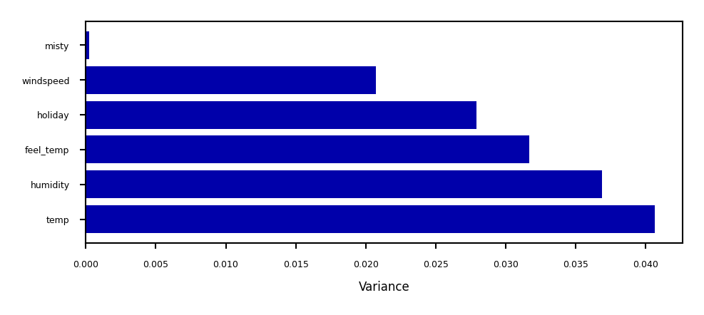
Unsupervised feature selection#
Variance-based
Remove (near) constant feature: choose a small variance threshold
Scale features before computing variance!
Infrequent values may still be important
Covariance-based
Remove correlated features
The small differences may actually be important
You don’t know because you don’t consider the target
from sklearn.feature_selection import f_regression, SelectPercentile, mutual_info_regression, SelectFromModel, RFE
from tqdm.notebook import trange, tqdm
from sklearn.preprocessing import scale
from sklearn.ensemble import RandomForestRegressor
from sklearn.pipeline import make_pipeline
from sklearn.model_selection import cross_val_score, GridSearchCV


# Pre-compute all importances on bike sharing dataset
# Scaled feature selection thresholds
thresholds = [0.25, 0.5, 0.75, 1]
# Dict to store all data
fs = {}
methods = ['FTest','MutualInformation']
for m in methods:
    fs[m] = {}
    fs[m]['select'] = {}
    fs[m]['cv_score'] = {}

def cv_score(selector):
    model = RandomForestRegressor()
    select_pipe = make_pipeline(StandardScaler(), selector, model)
    return np.mean(cross_val_score(select_pipe, X_bike, y_bike, cv=3))

# F test
print("Computing F test")
fs['FTest']['label'] = "F test"
fs['FTest']['score'] = f_regression(scale(X_bike),y_bike)[0]
fs['FTest']['scaled_score'] = fs['FTest']['score'] / np.max(fs['FTest']['score'])
for t in tqdm(thresholds):
    selector = SelectPercentile(score_func=f_regression, percentile=t*100).fit(scale(X_bike), y_bike)
    fs['FTest']['select'][t] = selector.get_support()
    fs['FTest']['cv_score'][t] = cv_score(selector)

# Mutual information
print("Computing Mutual information")
fs['MutualInformation']['label'] = "Mutual Information"
fs['MutualInformation']['score'] = mutual_info_regression(scale(X_bike),y_bike,discrete_features=range(13)) # first 13 features are discrete
fs['MutualInformation']['scaled_score'] = fs['MutualInformation']['score'] / np.max(fs['MutualInformation']['score'])
for t in tqdm(thresholds):
    selector = SelectPercentile(score_func=mutual_info_regression, percentile=t*100).fit(scale(X_bike), y_bike)
    fs['MutualInformation']['select'][t] = selector.get_support()
    fs['MutualInformation']['cv_score'][t] = cv_score(selector)

def plot_feature_importances(method1='f_test', method2=None, threshold=0.5):

    # Plot scores
    x = np.arange(20)
    fig, ax1 = plt.subplots(1, 1, figsize=(4*fig_scale, 1*fig_scale))
    w = 0.3
    imp = fs[method1]
    mask = imp['select'][threshold]
    m1 = ax1.bar(x[mask], imp['scaled_score'][mask], width=w, color='b', align='center')
    ax1.bar(x[~mask], imp['scaled_score'][~mask], width=w, color='b', align='center', alpha=0.3)
    if method2:
        imp2 = fs[method2]
        mask2 = imp2['select'][threshold]
        ax2 = ax1.twinx()
        m2 = ax2.bar(x[mask2] + w, imp2['scaled_score'][mask2], width=w,color='g',align='center')
        ax2.bar(x[~mask2] + w, imp2['scaled_score'][~mask2], width=w,color='g',align='center', alpha=0.3)
        plt.legend([m1, m2],['{} (Ridge R2:{:.2f})'.format(imp['label'],imp['cv_score'][threshold]),
                             '{} (Ridge R2:{:.2f})'.format(imp2['label'],imp2['cv_score'][threshold])], loc='upper left')
    else:
        plt.legend([m1],['{} (Ridge R2:{:.2f})'.format(imp['label'],imp['cv_score'][threshold])], loc='upper left')
    ax1.set_xticks(range(len(bike_names)))
    ax1.set_xticklabels(bike_names, rotation=45, ha="right");
    plt.title("Feature importance (selection threshold {:.2f})".format(threshold))

    plt.show()
Computing F test
Computing Mutual information
Show code cell source
from sklearn.feature_selection import VarianceThreshold
selector = VarianceThreshold().fit(MinMaxScaler().fit_transform(X_bike))
variances = selector.variances_
var_sort = np.argsort(variances)

plt.figure(figsize=(4*fig_scale, 1.5*fig_scale))
ypos = np.arange(6)[::-1]
plt.barh(ypos, variances[var_sort][:6], align='center')
plt.yticks(ypos, np.array(bike_names)[var_sort][:6])
plt.xlabel("Variance");
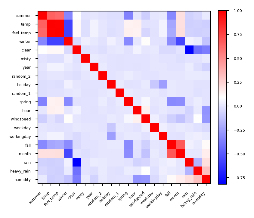
Covariance based feature selection#
Remove features \(X_i\) (= \(\mathbf{X_{:,i}}\)) that are highly correlated (have high correlation coefficient \(\rho\)) $\(\rho (X_1,X_2)={\frac {{\mathrm {cov}}(X_1,X_2)}{\sigma (X_1)\sigma (X_2)}} = {\frac { \frac{1}{N-1} \sum_i (X_{i,1} - \overline{X_1})(X_{i,2} - \overline{X_2}) }{\sigma (X_1)\sigma (X_2)}}\)$
Should we remove
feel_temp? Ortemp? Maybe one correlates more with the target?
Show code cell source
from sklearn.preprocessing import scale
from scipy.cluster import hierarchy

X_bike_scaled = scale(X_bike)
cov = np.cov(X_bike_scaled, rowvar=False)

order = np.array(hierarchy.dendrogram(hierarchy.ward(cov), no_plot=True)['ivl'], dtype="int")
bike_names_ordered = [bike_names[i] for i in order]

plt.figure(figsize=(3*fig_scale, 3*fig_scale))
plt.imshow(cov[order, :][:, order], cmap='bwr')
plt.xticks(range(X_bike.shape[1]), bike_names_ordered, ha="right")
plt.yticks(range(X_bike.shape[1]), bike_names_ordered)
plt.xticks(rotation=45)
plt.colorbar(fraction=0.046, pad=0.04);
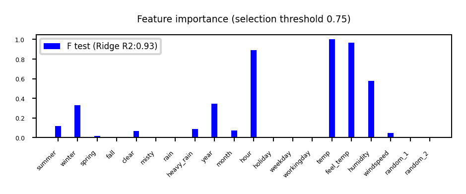
Univariate statistics (F-test)#
Consider each feature individually (univariate), independent of the model that you aim to apply
Use a statistical test: is there a linear statistically significant relationship with the target?
Use F-statistic (or corresponding p value) to rank all features, then select features using a threshold
Best \(k\), best \(k\) %, probability of removing useful features (FPR),…
Cannot detect correlations (e.g. temp and feel_temp) or interactions (e.g. binary features)
Show code cell source
plot_feature_importances('FTest', None, threshold=0.75)
F-statistic#
For regression: does feature \(X_i\) correlate (positively or negatively) with the target \(y\)? $\(\text{F-statistic} = \frac{\rho(X_i,y)^2}{1-\rho(X_i,y)^2} \cdot (N-1)\)$
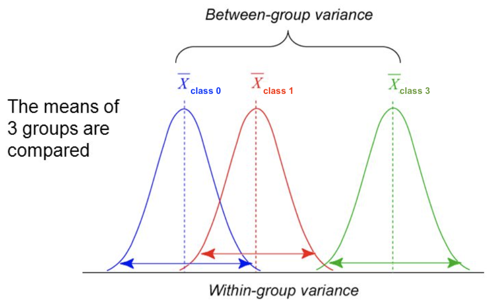
For classification: uses ANOVA: does \(X_i\) explain the between-class variance?
Alternatively, use the \(\chi^2\) test (only for categorical features) $\(\text{F-statistic} = \frac{\text{within-class variance}}{\text{between-class variance}} =\frac{var(\overline{X_i})}{\overline{var(X_i)}}\)$
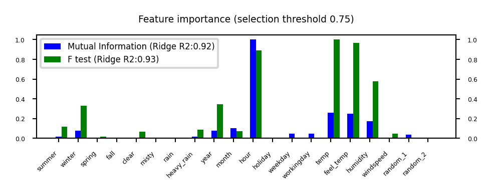
Mutual information#
Measures how much information \(X_i\) gives about the target \(Y\). In terms of entropy \(H\): $\(MI(X,Y) = H(X) + H(Y) - H(X,Y)\)$
Idea: estimate H(X) as the average distance between a data point and its \(k\) Nearest Neighbors
You need to choose \(k\) and say which features are categorical
Captures complex dependencies (e.g. hour, month), but requires more samples to be accurate
Show code cell source
plot_feature_importances('MutualInformation', 'FTest', threshold=0.75)
Further techniques#
Many more powerful techniques exist
Model-based: Random Forests, Linear models, kNN
Wrapping techniques (black-box search)
Permutation importance
See the Data Preprocessing lecture.
Feature Engineering#
Create new features based on existing ones
Polynomial features
Interaction features
Binning
Mainly useful for simple models (e.g. linear models)
Other models can learn interations themselves
But may be slower, less robust than linear models
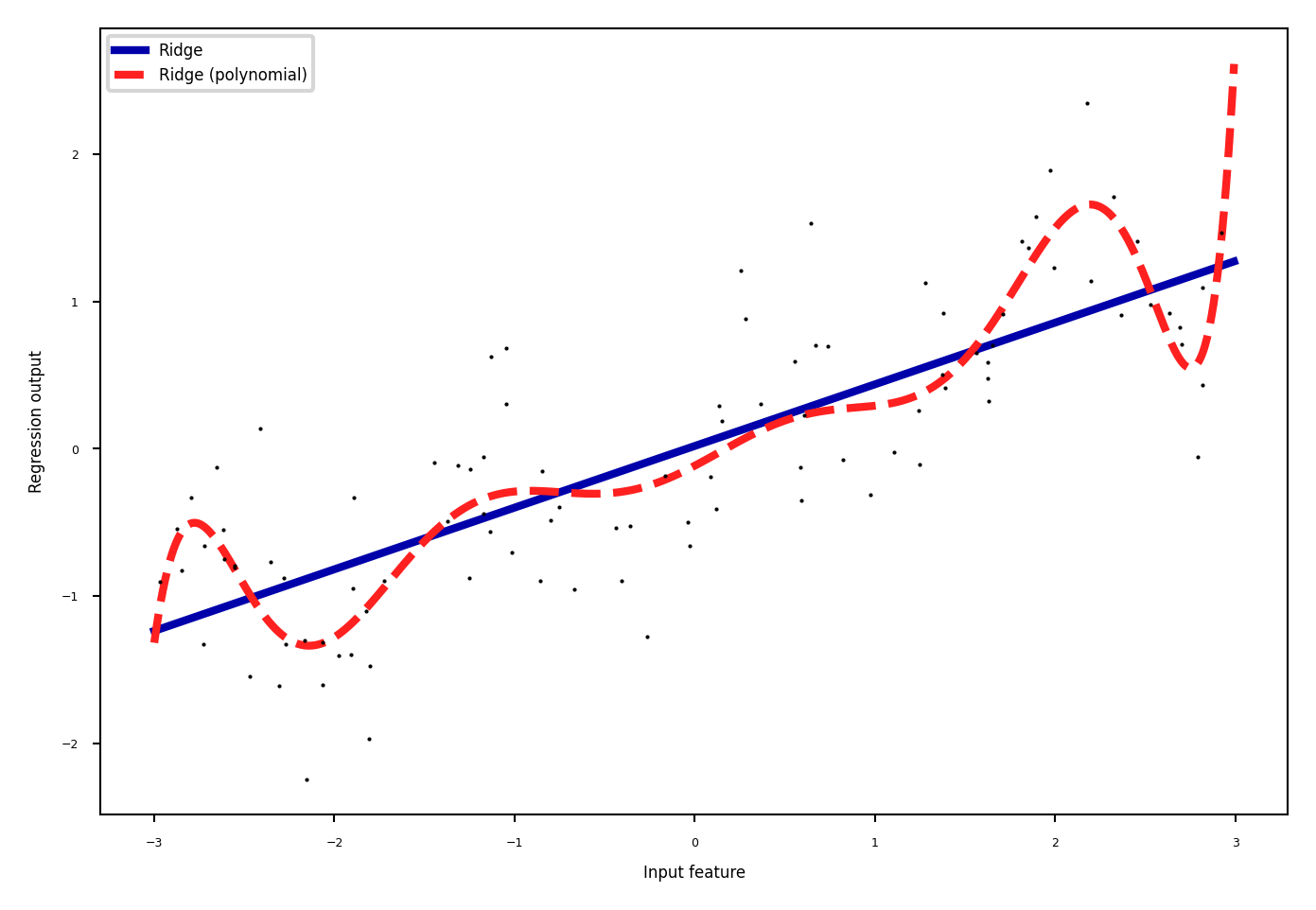
Polynomials#
Add all polynomials up to degree \(d\) and all products
Equivalent to polynomial basis expansions $\([1, x_1, ..., x_p] \xrightarrow{} [1, x_1, ..., x_p, x_1^2, ..., x_p^2, ..., x_p^d, x_1 x_2, ..., x_{p-1} x_p]\)$
Show code cell source
from sklearn.linear_model import LinearRegression, Ridge
from sklearn.tree import DecisionTreeRegressor
from sklearn.preprocessing import PolynomialFeatures

# Wavy data
X, y = mglearn.datasets.make_wave(n_samples=100)
line = np.linspace(-3, 3, 1000, endpoint=False).reshape(-1, 1)

# Normal ridge
lreg = Ridge().fit(X, y)
plt.rcParams['figure.figsize'] = [6*fig_scale, 4*fig_scale]
plt.plot(line, lreg.predict(line), lw=2, label="Ridge")

# include polynomials up to x ** 10
poly = PolynomialFeatures(degree=10, include_bias=False)
X_poly = poly.fit_transform(X)
preg = Ridge().fit(X_poly, y)
line_poly = poly.transform(line)
plt.plot(line, preg.predict(line_poly), lw=2, label='Ridge (polynomial)')

plt.plot(X[:, 0], y, 'o', c='k')
plt.ylabel("Regression output")
plt.xlabel("Input feature")
plt.legend(loc="best");
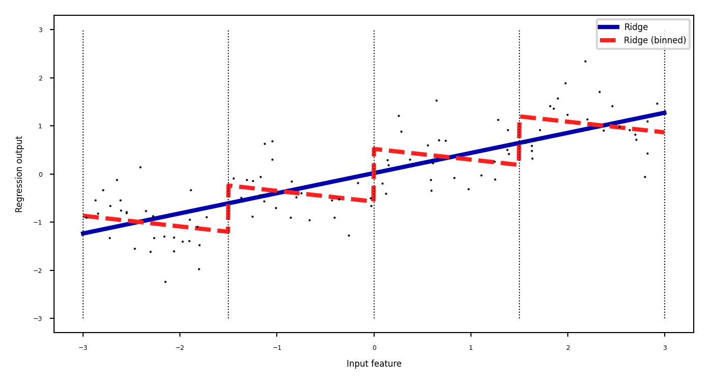
Binning#
Partition numeric feature values into \(n\) intervals (bins)
Create \(n\) new one-hot features, 1 if original value falls in corresponding bin
Models different intervals differently (e.g. different age groups)
table_font_size = 20
heading_properties = [('font-size', table_font_size)]
cell_properties = [('font-size', table_font_size)]
dfstyle = [dict(selector="th", props=heading_properties),\
 dict(selector="td", props=cell_properties)]
Show code cell source
from sklearn.preprocessing import OneHotEncoder

# create 11 equal bins
bins = np.linspace(-3, 3, 5)
# assign to bins
which_bin = np.digitize(X, bins=bins)
# transform using the OneHotEncoder.
encoder = OneHotEncoder(sparse_output=False)
# encoder.fit finds the unique values that appear in which_bin
encoder.fit(which_bin)
# transform creates the one-hot encoding
X_binned = encoder.transform(which_bin)
# Plot transformed data
bin_names = [('[%.1f,%.1f]') % i for i in zip(bins, bins[1:])]
df_orig = pd.DataFrame(X, columns=["orig"])
df_nr = pd.DataFrame(which_bin, columns=["which_bin"])
# add the original features
X_combined = np.hstack([X, X_binned])
ohedf = pd.DataFrame(X_combined, columns=["orig"]+bin_names).head(3)
ohedf.style.set_table_styles(dfstyle)
| orig | [-3.0,-1.5] | [-1.5,0.0] | [0.0,1.5] | [1.5,3.0] | |
|---|---|---|---|---|---|
| 0 | -0.752759 | 0.000000 | 1.000000 | 0.000000 | 0.000000 |
| 1 | 2.704286 | 0.000000 | 0.000000 | 0.000000 | 1.000000 |
| 2 | 1.391964 | 0.000000 | 0.000000 | 1.000000 | 0.000000 |
Show code cell source
line_binned = encoder.transform(np.digitize(line, bins=bins))
reg = LinearRegression().fit(X_combined, y)

line_combined = np.hstack([line, line_binned])

plt.rcParams['figure.figsize'] = [6*fig_scale, 3*fig_scale]
plt.plot(line, lreg.predict(line), lw=2, label="Ridge")
plt.plot(line, reg.predict(line_combined), lw=2, label='Ridge (binned)')

for bin in bins:
    plt.plot([bin, bin], [-3, 3], ':', c='k')
plt.legend(loc="best")
plt.ylabel("Regression output")
plt.xlabel("Input feature")
plt.plot(X[:, 0], y, 'o', c='k');
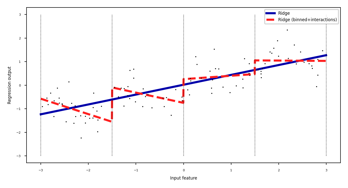
Binning + interaction features#
Add interaction features (or product features )
Product of the bin encoding and the original feature value
Learn different weights per bin
Show code cell source
X_product = np.hstack([X_binned, X * X_binned])
bin_sname = ["b" + str(s) for s in range(4)]
X_combined = np.hstack([X, X_product])
pd.set_option('display.max_columns', 10)
bindf = pd.DataFrame(X_combined, columns=["orig"]+bin_sname+["X*" + s for s in bin_sname]).head(3)
bindf.style.set_table_styles(dfstyle)
| orig | b0 | b1 | b2 | b3 | X*b0 | X*b1 | X*b2 | X*b3 | |
|---|---|---|---|---|---|---|---|---|---|
| 0 | -0.752759 | 0.000000 | 1.000000 | 0.000000 | 0.000000 | -0.000000 | -0.752759 | -0.000000 | -0.000000 |
| 1 | 2.704286 | 0.000000 | 0.000000 | 0.000000 | 1.000000 | 0.000000 | 0.000000 | 0.000000 | 2.704286 |
| 2 | 1.391964 | 0.000000 | 0.000000 | 1.000000 | 0.000000 | 0.000000 | 0.000000 | 1.391964 | 0.000000 |
Show code cell source
reg = LinearRegression().fit(X_product, y)

line_product = np.hstack([line_binned, line * line_binned])
plt.plot(line, lreg.predict(line), lw=2, label="Ridge")
plt.plot(line, reg.predict(line_product), lw=2, label='Ridge (binned+interactions)')

for bin in bins:
    plt.plot([bin, bin], [-3, 3], ':', c='k')

plt.plot(X[:, 0], y, 'o', c='k')
plt.ylabel("Regression output")
plt.xlabel("Input feature")
plt.legend(loc="best");
Categorical feature interactions#
One-hot-encode categorical feature
Multiply every one-hot-encoded column with every numeric feature
Allows to built different submodels for different categories
Show code cell source
df = pd.DataFrame({'gender': ['M', 'F', 'M', 'F', 'F'],
                   'age': [14, 16, 12, 25, 22],
                   'pageviews': [70, 12, 42, 64, 93],
                   'time': [269, 1522, 235, 63, 21]
                  })
df.head(3)
df.style.set_table_styles(dfstyle)
| gender | age | pageviews | time | |
|---|---|---|---|---|
| 0 | M | 14 | 70 | 269 |
| 1 | F | 16 | 12 | 1522 |
| 2 | M | 12 | 42 | 235 |
| 3 | F | 25 | 64 | 63 |
| 4 | F | 22 | 93 | 21 |
Show code cell source
dummies = pd.get_dummies(df)
df_f = dummies.multiply(dummies.gender_F, axis='rows')
df_f = df_f.rename(columns=lambda x: x + "_F")
df_m = dummies.multiply(dummies.gender_M, axis='rows')
df_m = df_m.rename(columns=lambda x: x + "_M")
res = pd.concat([df_m, df_f], axis=1).drop(["gender_F_M", "gender_M_F"], axis=1)
res.head(3)
res.style.set_table_styles(dfstyle)
| age_M | pageviews_M | time_M | gender_M_M | age_F | pageviews_F | time_F | gender_F_F | |
|---|---|---|---|---|---|---|---|---|
| 0 | 14 | 70 | 269 | True | 0 | 0 | 0 | False |
| 1 | 0 | 0 | 0 | False | 16 | 12 | 1522 | True |
| 2 | 12 | 42 | 235 | True | 0 | 0 | 0 | False |
| 3 | 0 | 0 | 0 | False | 25 | 64 | 63 | True |
| 4 | 0 | 0 | 0 | False | 22 | 93 | 21 | True |
Summary#
Data preprocessing is a crucial part of machine learning
Scaling is important for many distance-based methods (e.g. kNN, SVM, Neural Nets)
Selecting features can speed up models and reduce overfitting
Feature engineering is often useful for linear models
Many more techniques (e.g. missing value imputation, handling data imbalance,…) will be discussed in the data preprocessing lecture
Pipelines allow us to encapsulate multiple steps in a convenient way
Avoids data leakage, crucial for proper evaluation
Choose the right preprocessing steps and models in your pipeline
Cross-validation helps, but the search space is huge
Smarter techniques exist to automate this process (i.e. AutoML)