Lab 1: Machine Learning with Python

Lab 1: Machine Learning with Python#

Joaquin Vanschoren, Pieter Gijsbers, Bilge Celik, Prabhant Singh

%matplotlib inline
import numpy as np
import pandas as pd

Overview#

Why Python?
Intro to scikit-learn
Exercises

Why Python?#

Many data-heavy applications are now developed in Python
Highly readable, less complexity, fast prototyping
Easy to offload number crunching to underlying C/Fortran/…
Easy to install and import many rich libraries
- numpy: efficient data structures
- scipy: fast numerical recipes
- matplotlib: high-quality graphs
- scikit-learn: machine learning algorithms
- tensorflow: neural networks
- …

Numpy, Scipy, Matplotlib#

See the tutorials (in the course GitHub)
Many good tutorials online

scikit-learn#

One of the most prominent Python libraries for machine learning:

Contains many state-of-the-art machine learning algorithms
Builds on numpy (fast), implements advanced techniques
Wide range of evaluation measures and techniques
Offers comprehensive documentation about each algorithm
Widely used, and a wealth of tutorials and code snippets are available
Works well with numpy, scipy, pandas, matplotlib,…

Algorithms#

See the Reference

Supervised learning:

Linear models (Ridge, Lasso, Elastic Net, …)
Support Vector Machines
Tree-based methods (Classification/Regression Trees, Random Forests,…)
Nearest neighbors
Neural networks
Gaussian Processes
Feature selection

Unsupervised learning:

Clustering (KMeans, …)
Matrix Decomposition (PCA, …)
Manifold Learning (Embeddings)
Density estimation
Outlier detection

Model selection and evaluation:

Cross-validation
Grid-search
Lots of metrics

Data import#

Multiple options:

A few toy datasets are included in sklearn.datasets
Import 1000s of datasets via sklearn.datasets.fetch_openml
You can import data files (CSV) with pandas or numpy

from sklearn.datasets import load_iris, fetch_openml
iris_data = load_iris()
dating_data = fetch_openml("SpeedDating", version=1)

/Users/jvanscho/miniconda3/lib/python3.10/site-packages/sklearn/datasets/_openml.py:932: FutureWarning: The default value of `parser` will change from `'liac-arff'` to `'auto'` in 1.4. You can set `parser='auto'` to silence this warning. Therefore, an `ImportError` will be raised from 1.4 if the dataset is dense and pandas is not installed. Note that the pandas parser may return different data types. See the Notes Section in fetch_openml's API doc for details.
  warn(

These will return a Bunch object (similar to a dict)

print("Keys of iris_dataset: {}".format(iris_data.keys()))
print(iris_data['DESCR'][:193] + "\n...")

Keys of iris_dataset: dict_keys(['data', 'target', 'frame', 'target_names', 'DESCR', 'feature_names', 'filename', 'data_module'])
.. _iris_dataset:

Iris plants dataset
--------------------

**Data Set Characteristics:**

    :Number of Instances: 150 (50 in each of three classes)
    :Number of Attributes: 4 numeric, pre
...

Targets (classes) and features are lists of strings
Data and target values are always numeric (ndarrays)

print("Targets: {}".format(iris_data['target_names']))
print("Features: {}".format(iris_data['feature_names']))
print("Shape of data: {}".format(iris_data['data'].shape))
print("First 5 rows:\n{}".format(iris_data['data'][:5]))
print("Targets:\n{}".format(iris_data['target']))

Targets: ['setosa' 'versicolor' 'virginica']
Features: ['sepal length (cm)', 'sepal width (cm)', 'petal length (cm)', 'petal width (cm)']
Shape of data: (150, 4)
First 5 rows:
[[5.1 3.5 1.4 0.2]
 [4.9 3.  1.4 0.2]
 [4.7 3.2 1.3 0.2]
 [4.6 3.1 1.5 0.2]
 [5.  3.6 1.4 0.2]]
Targets:
[0 0 0 0 0 0 0 0 0 0 0 0 0 0 0 0 0 0 0 0 0 0 0 0 0 0 0 0 0 0 0 0 0 0 0 0 0
 0 0 0 0 0 0 0 0 0 0 0 0 0 1 1 1 1 1 1 1 1 1 1 1 1 1 1 1 1 1 1 1 1 1 1 1 1
 1 1 1 1 1 1 1 1 1 1 1 1 1 1 1 1 1 1 1 1 1 1 1 1 1 1 2 2 2 2 2 2 2 2 2 2 2
 2 2 2 2 2 2 2 2 2 2 2 2 2 2 2 2 2 2 2 2 2 2 2 2 2 2 2 2 2 2 2 2 2 2 2 2 2
 2 2]

Building models#

All scikitlearn estimators follow the same interface

class SupervisedEstimator(...):
    def __init__(self, hyperparam, ...):

    def fit(self, X, y):   # Fit/model the training data
        ...                # given data X and targets y
        return self
     
    def predict(self, X):  # Make predictions
        ...                # on unseen data X  
        return y_pred
    
    def score(self, X, y): # Predict and compare to true
        ...                # labels y                
        return score

Training and testing data#

To evaluate our classifier, we need to test it on unseen data.
train_test_split: splits data randomly in 75% training and 25% test data.

from sklearn.model_selection import train_test_split
X_train, X_test, y_train, y_test = train_test_split(
    iris_data['data'], iris_data['target'], 
    random_state=0)
print("X_train shape: {}".format(X_train.shape))
print("y_train shape: {}".format(y_train.shape))
print("X_test shape: {}".format(X_test.shape))
print("y_test shape: {}".format(y_test.shape))

X_train shape: (112, 4)
y_train shape: (112,)
X_test shape: (38, 4)
y_test shape: (38,)

We can also choose other ways to split the data. For instance, the following will create a training set of 10% of the data and a test set of 5% of the data. This is useful when dealing with very large datasets. stratify defines the target feature to stratify the data (ensure that the class distributions are kept the same).

X, y = iris_data['data'], iris_data['target']
Xs_train, Xs_test, ys_train, ys_test = train_test_split(X,y, stratify=y, train_size=0.1, test_size=0.05)
print("Xs_train shape: {}".format(Xs_train.shape))
print("Xs_test shape: {}".format(Xs_test.shape))

Xs_train shape: (15, 4)
Xs_test shape: (8, 4)

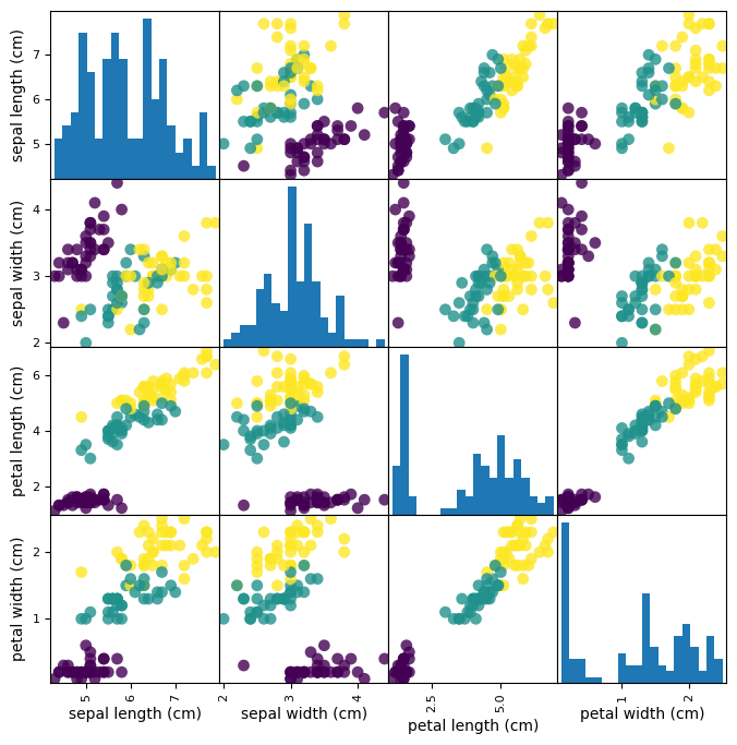
Looking at your data (with pandas)#

from pandas.plotting import scatter_matrix

# Build a DataFrame with training examples and feature names
iris_df = pd.DataFrame(X_train, 
                       columns=iris_data.feature_names)

# scatter matrix from the dataframe, color by class
sm = scatter_matrix(iris_df, c=y_train, figsize=(8, 8), 
                  marker='o', hist_kwds={'bins': 20}, s=60, 
                  alpha=.8)

../_images/10d24ce085ada3e2a9e8e3407e1da5b7f82b19fc7f7eb8ea1ffd69e9635faecc.png

Fitting a model#

The first model we’ll build is a k-Nearest Neighbor classifier.
kNN is included in sklearn.neighbors, so let’s build our first model

from sklearn.neighbors import KNeighborsClassifier
knn = KNeighborsClassifier(n_neighbors=1)
knn.fit(X_train, y_train)

KNeighborsClassifier(n_neighbors=1)

In a Jupyter environment, please rerun this cell to show the HTML representation or trust the notebook.
On GitHub, the HTML representation is unable to render, please try loading this page with nbviewer.org.

Making predictions#

Let’s create a new example and ask the kNN model to classify it

X_new = np.array([[5, 2.9, 1, 0.2]])
prediction = knn.predict(X_new)
print("Prediction: {}".format(prediction))
print("Predicted target name: {}".format(
       iris_data['target_names'][prediction]))

Prediction: [0]
Predicted target name: ['setosa']

Evaluating the model#

Feeding all test examples to the model yields all predictions

y_pred = knn.predict(X_test)
print("Test set predictions:\n {}".format(y_pred))

Test set predictions:
 [2 1 0 2 0 2 0 1 1 1 2 1 1 1 1 0 1 1 0 0 2 1 0 0 2 0 0 1 1 0 2 1 0 2 2 1 0
 2]

The score function computes the percentage of correct predictions

knn.score(X_test, y_test)

print("Score: {:.2f}".format(knn.score(X_test, y_test) ))

Score: 0.97

Instead of a single train-test split, we can use cross_validate do run a cross-validation. It will return the test scores, as well as the fit and score times, for every fold. By default, scikit-learn does a 5-fold cross-validation, hence returning 5 test scores.

!pip install -U joblib

Requirement already satisfied: joblib in /Users/jvanscho/miniconda3/lib/python3.10/site-packages (1.2.0)

from sklearn.model_selection import cross_validate
xval = cross_validate(knn, X, y, return_train_score=True, n_jobs=-1)
xval

{'fit_time': array([0.0004108 , 0.00043321, 0.00047421, 0.00054502, 0.00044918]),
 'score_time': array([0.00080895, 0.00081778, 0.00089979, 0.00099206, 0.00093198]),
 'test_score': array([0.96666667, 0.96666667, 0.93333333, 0.93333333, 1.        ]),
 'train_score': array([1., 1., 1., 1., 1.])}

The mean should give a better performance estimate

np.mean(xval['test_score'])

0.96

Introspecting the model#

Most models allow you to retrieve the trained model parameters, usually called coef_

from sklearn.linear_model import LinearRegression
lr = LinearRegression().fit(X_train, y_train)
lr.coef_

array([-0.15330146, -0.02540761,  0.26698013,  0.57386186])

Matching these with the names of the features, we can see which features are primarily used by the model

d = zip(iris_data.feature_names,lr.coef_)
set(d)

{('petal length (cm)', 0.2669801292888399),
 ('petal width (cm)', 0.5738618608875331),
 ('sepal length (cm)', -0.15330145645467938),
 ('sepal width (cm)', -0.025407610745503684)}

Please see the course notebooks for more examples on how to analyse models.