Lecture 9: Convolutional Neural Networks

Handling image data

Joaquin Vanschoren, Eindhoven University of Technology

Overview

• Image convolution
• Convolutional neural networks
• Data augmentation
• Model interpretation
• Using pre-trained networks (transfer learning)

Convolutions

• Operation that transforms an image by sliding a smaller image (called a filter or kernel ) over the image and multiplying the pixel values
  • Slide an $n$ x $n$ filter over $n$ x $n$ patches of the original image
  • Every pixel is replaced by the sum of the element-wise products of the values of the image patch around that pixel and the kernel

# kernel and image_patch are n x n matrices
pixel_out = np.sum(kernel * image_patch)

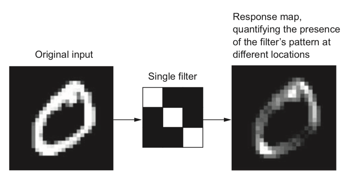
• Different kernels can detect different types of patterns in the image

interactive(children=(IntSlider(value=0, description='i_step', max=783), Output()), _dom_classes=('widget-inte…

<generator object iter_kernel_labels at 0x2cca0c2e0>
<generator object iter_kernel_labels at 0x2cca0c2e0>
<generator object iter_kernel_labels at 0x2cca0c2e0>

Demonstration on Google streetview data

House numbers photographed from Google streetview imagery, cropped and centered around digits, but with neighboring numbers or other edge artifacts.

For recognizing digits, color is not important, so we grayscale the images

Demonstration

interactive(children=(IntSlider(value=0, description='i_step', max=1023), Output()), _dom_classes=('widget-int…

<generator object iter_kernel_labels at 0x2cca0f680>
<generator object iter_kernel_labels at 0x2cca0f680>
<generator object iter_kernel_labels at 0x2cca0f680>

Image convolution in practice

• How do we know which filters are best for a given image?
• Families of kernels (or filter banks ) can be run on every image
  • Gabor, Sobel, Haar Wavelets,...
• Gabor filters: Wave patterns generated by changing:
  • Frequency: narrow or wide ondulations
  • Theta: angle (direction) of the wave
  • Sigma: resolution (size of the filter)

Demonstration

interactive(children=(FloatSlider(value=0.46, description='frequency', max=1.0, min=0.01, step=0.05), FloatSli…

Demonstration on the streetview data

interactive(children=(FloatSlider(value=0.46, description='frequency', max=1.0, min=0.01, step=0.05), FloatSli…

Filter banks

• Different filters detect different edges, shapes,...
• Not all seem useful

Another example: Fashion MNIST

Demonstration

interactive(children=(FloatSlider(value=0.46, description='frequency', max=1.0, min=0.01, step=0.05), FloatSli…

Fashion MNIST with multiple filters (filter bank)

Convolutional neural nets

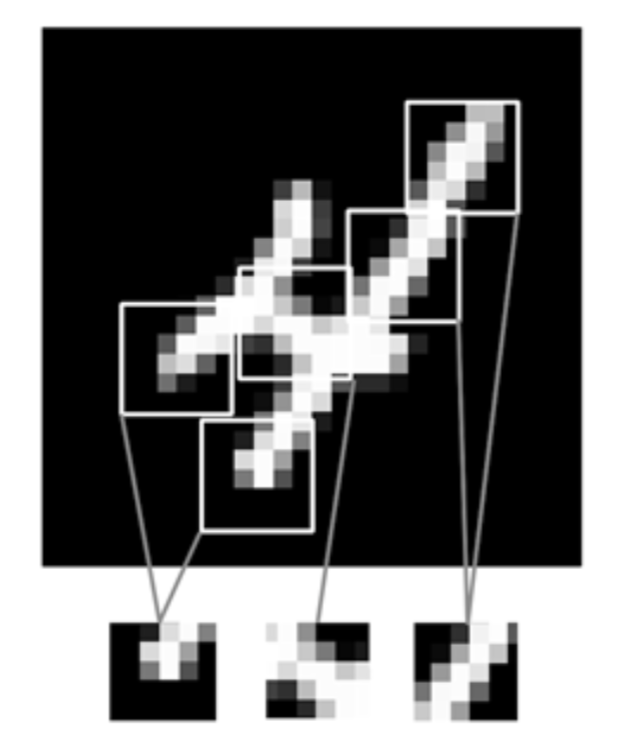
• Finding relationships between individual pixels and the correct class is hard
• We want to discover 'local' patterns (edges, lines, endpoints)
• Representing such local patterns as features makes it easier to learn from them
• We could use convolutions, but how to choose the filters?

Convolutional Neural Networks (ConvNets)

• Instead of manually designing the filters, we can also learn them based on data
  • Choose filter sizes (manually), initialize with small random weights
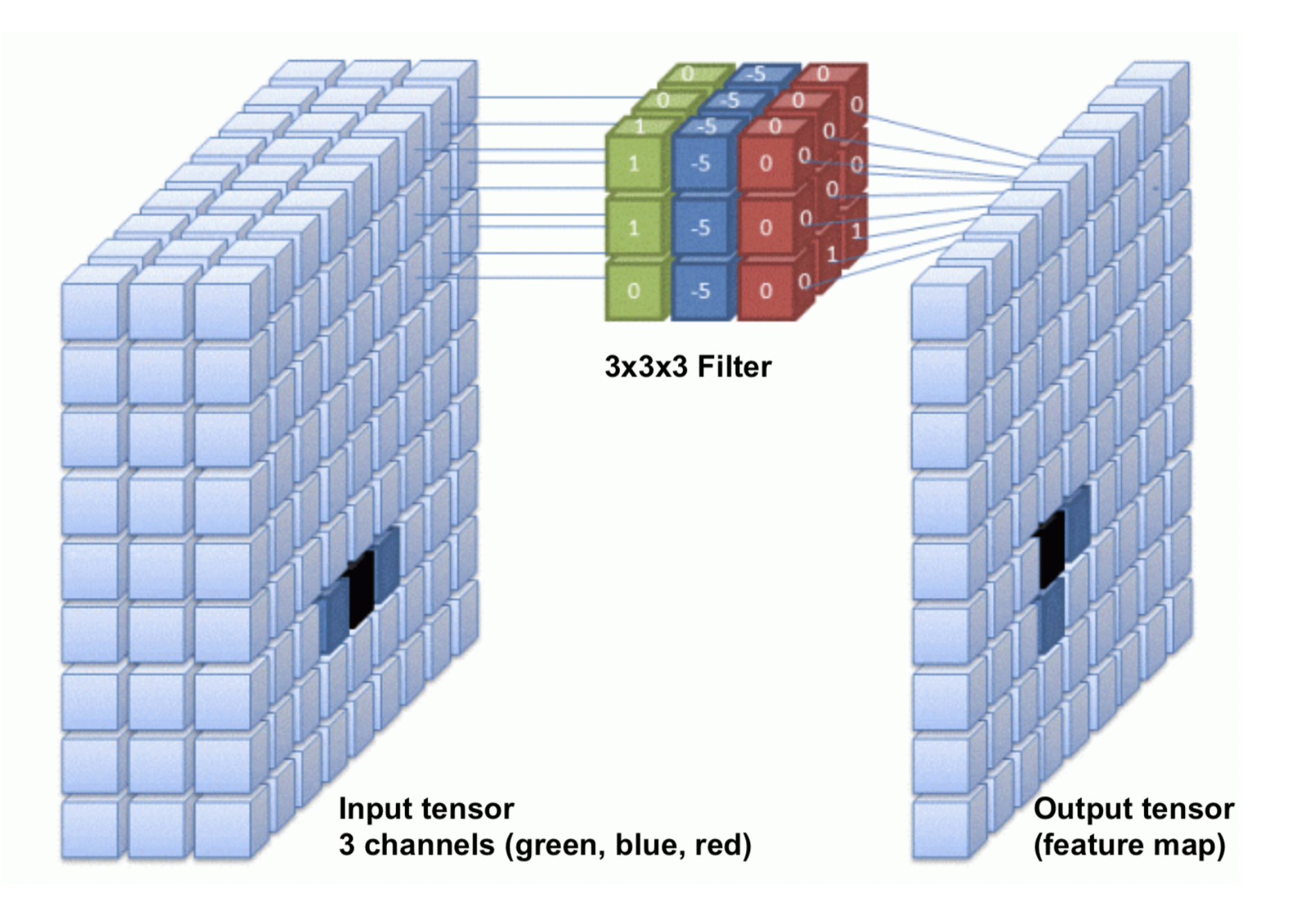
• Forward pass: Convolutional layer slides the filter over the input, generates the output
• Backward pass: Update the filter weights according to the loss gradient
• Illustration for 1 filter:

Convolutional layers: Feature maps

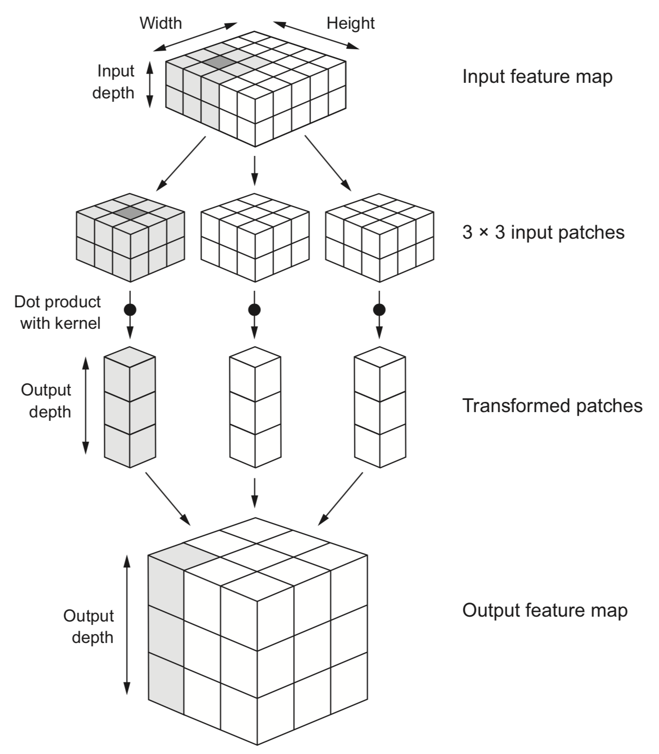
• One filter is not sufficient to detect all relevant patterns in an image
• A convolutional layer applies and learns $d$ filter in parallel
• Slide $d$ filters across the input image (in parallel) -> a (1x1xd) output per patch
• Reassemble into a feature map with $d$ 'channels', a (width x height x d) tensor.

Border effects (zero padding)

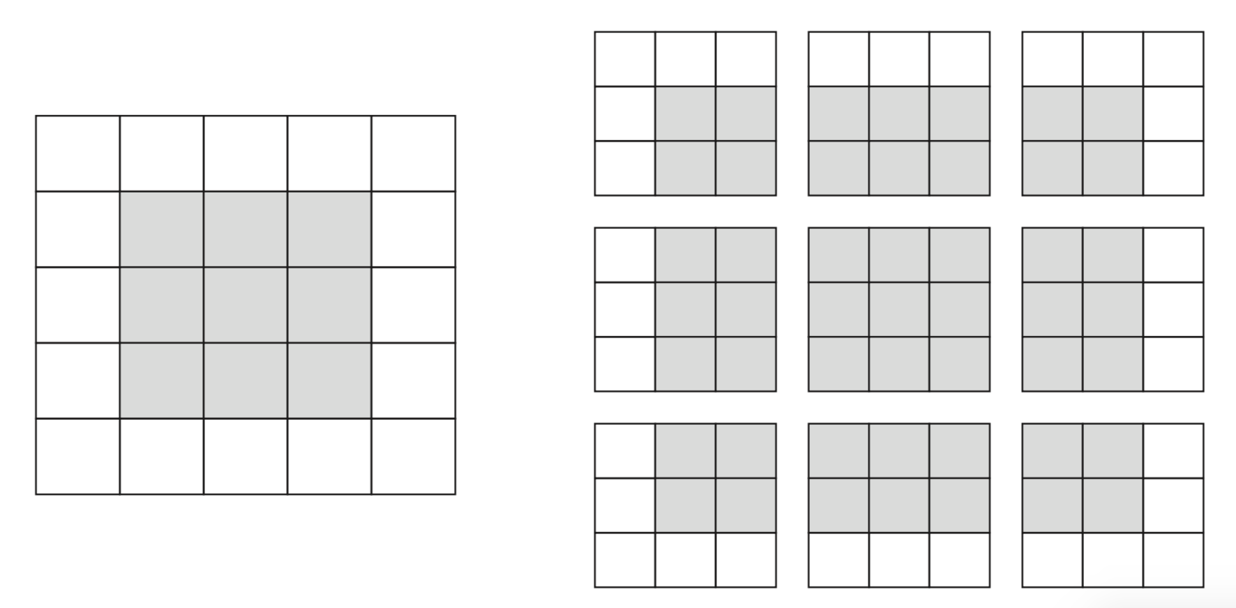
• Consider a 5x5 image and a 3x3 filter: there are only 9 possible locations, hence the output is a 3x3 feature map
• If we want to maintain the image size, we use zero-padding, adding 0's all around the input tensor.

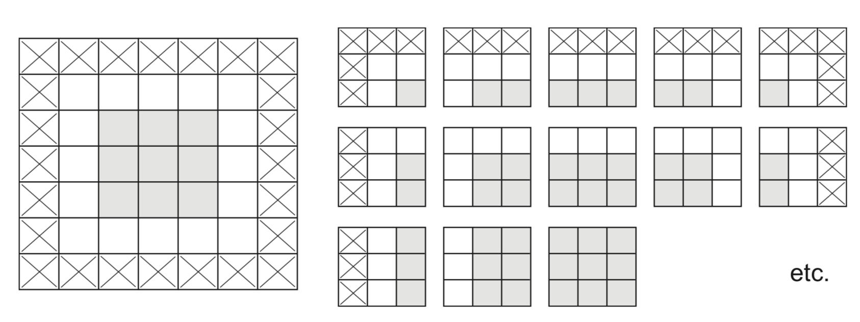
Undersampling (striding)

• Sometimes, we want to downsample a high-resolution image
  • Faster processing, less noisy (hence less overfitting)
• One approach is to skip values during the convolution
  • Distance between 2 windows: stride length
• Example with stride length 2 (without padding):

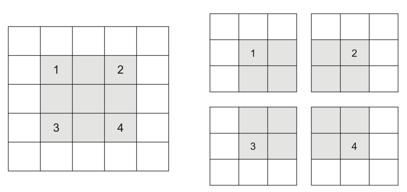
Max-pooling

• Another approach to shrink the input tensors is max-pooling :
  • Run a filter with a fixed stride length over the image
    • Usually 2x2 filters and stride lenght 2
  • The filter simply returns the max (or avg ) of all values
• Agressively reduces the number of weights (less overfitting)
• Information from every input node spreads more quickly to output nodes
  • In pure convnets, one input value spreads to 3x3 nodes of the first layer, 5x5 nodes of the second, etc.
  • Without maxpooling, you need much deeper networks, harder to train
• Increases translation invariance : patterns can affect the predictions no matter where they occur in the image

Convolutional nets in practice

• Use multiple convolutional layers to learn patterns at different levels of abstraction
  • Find local patterns first (e.g. edges), then patterns across those patterns
• Use MaxPooling layers to reduce resolution, increase translation invariance
• Use sufficient filters in the first layer (otherwise information gets lost)
• In deeper layers, use increasingly more filters
  • Preserve information about the input as resolution descreases
  • Avoid decreasing the number of activations (resolution x nr of filters)
• For very deep nets, add skip connections to preserve information (and gradients)
  • Sums up outputs of earlier layers to those of later layers (with same dimensions)

Example with Keras

• Conv2D for 2D convolutional layers
  • 32 filters (default), randomly initialized (from uniform distribution)
  • Deeper layers use 64 filters
  • Filter size is 3x3
  • ReLU activation to simplify training of deeper networks
• MaxPooling2D for max-pooling
  • 2x2 pooling reduces the number of inputs by a factor 4

model = models.Sequential()
model.add(layers.Conv2D(32, (3, 3), activation='relu', 
                        input_shape=(28, 28, 1)))
model.add(layers.MaxPooling2D((2, 2)))
model.add(layers.Conv2D(64, (3, 3), activation='relu'))
model.add(layers.MaxPooling2D((2, 2)))
model.add(layers.Conv2D(64, (3, 3), activation='relu'))

Observe how the input image on 28x28x1 is transformed to a 3x3x64 feature map

• Convolutional layer:
  • No zero-padding: every output 2 pixels less in every dimension
  • 320 weights: (3x3 filter weights + 1 bias) * 32 filters
• After every MaxPooling, resolution halved in every dimension

Model: "sequential"
_________________________________________________________________
 Layer (type)                Output Shape              Param #   
=================================================================
 conv2d (Conv2D)             (None, 26, 26, 32)        320       
                                                                 
 max_pooling2d (MaxPooling2D  (None, 13, 13, 32)       0         
 )                                                               
                                                                 
 conv2d_1 (Conv2D)           (None, 11, 11, 64)        18496     
                                                                 
 max_pooling2d_1 (MaxPooling  (None, 5, 5, 64)         0         
 2D)                                                             
                                                                 
 conv2d_2 (Conv2D)           (None, 3, 3, 64)          36928     
                                                                 
=================================================================
Total params: 55,744
Trainable params: 55,744
Non-trainable params: 0
_________________________________________________________________

• To classify the images, we still need a Dense and Softmax layer.
• We can flatten the 3x3x64 feature map to a vector of size 576

model.add(layers.Flatten())
model.add(layers.Dense(64, activation='relu'))
model.add(layers.Dense(10, activation='softmax'))

Model: "sequential"
_________________________________________________________________
 Layer (type)                Output Shape              Param #   
=================================================================
 conv2d (Conv2D)             (None, 26, 26, 32)        320       
                                                                 
 max_pooling2d (MaxPooling2D  (None, 13, 13, 32)       0         
 )                                                               
                                                                 
 conv2d_1 (Conv2D)           (None, 11, 11, 64)        18496     
                                                                 
 max_pooling2d_1 (MaxPooling  (None, 5, 5, 64)         0         
 2D)                                                             
                                                                 
 conv2d_2 (Conv2D)           (None, 3, 3, 64)          36928     
                                                                 
 flatten (Flatten)           (None, 576)               0         
                                                                 
 dense (Dense)               (None, 64)                36928     
                                                                 
 dense_1 (Dense)             (None, 10)                650       
                                                                 
=================================================================
Total params: 93,322
Trainable params: 93,322
Non-trainable params: 0
_________________________________________________________________

• Flatten adds a lot of weights
• Instead, we can do GlobalAveragePooling: returns average of each activation map
• This sometimes works even without adding a dense layer (the number of outputs is similar to the number of classes)

model.add(layers.GlobalAveragePooling2D())
model.add(layers.Dense(10, activation='softmax'))

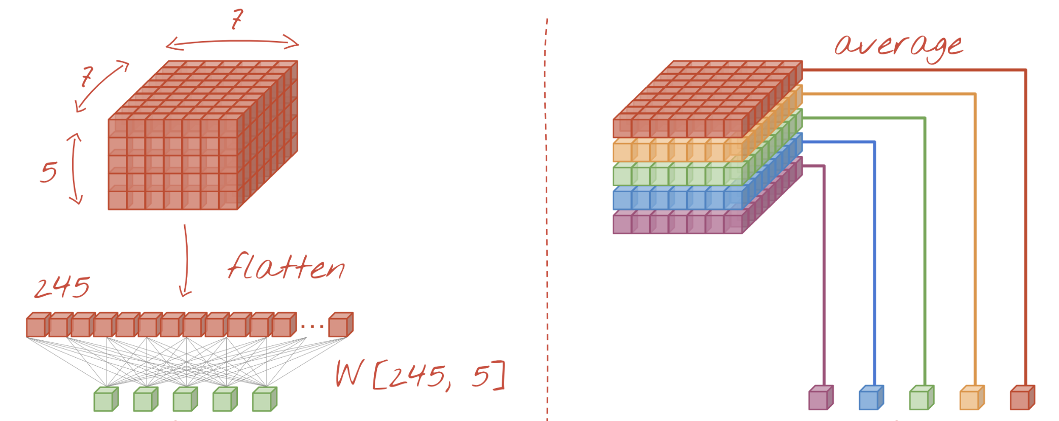
• With GlobalAveragePooling: much fewer weights to learn
• Use with caution: this destroys the location information learned by the CNN
• Not ideal for tasks such as object localization

Model: "sequential_1"
_________________________________________________________________
 Layer (type)                Output Shape              Param #   
=================================================================
 conv2d_3 (Conv2D)           (None, 26, 26, 32)        320       
                                                                 
 max_pooling2d_2 (MaxPooling  (None, 13, 13, 32)       0         
 2D)                                                             
                                                                 
 conv2d_4 (Conv2D)           (None, 11, 11, 64)        18496     
                                                                 
 max_pooling2d_3 (MaxPooling  (None, 5, 5, 64)         0         
 2D)                                                             
                                                                 
 conv2d_5 (Conv2D)           (None, 3, 3, 64)          36928     
                                                                 
 global_average_pooling2d (G  (None, 64)               0         
 lobalAveragePooling2D)                                          
                                                                 
 dense_2 (Dense)             (None, 10)                650       
                                                                 
=================================================================
Total params: 56,394
Trainable params: 56,394
Non-trainable params: 0
_________________________________________________________________

Run the model on MNIST dataset

• Train and test as usual: 99% accuracy
  • Compared to 97,8% accuracy with the dense architecture
  • Flatten and GlobalAveragePooling yield similar performance

Accuracy:  0.988800048828125

Tip:

• Training ConvNets can take a lot of time
• Save the trained model (and history) to disk so that you can reload it later

model.save(os.path.join(model_dir, 'mnist.h5'))
with open(os.path.join(model_dir, 'mnist_history.p'), 'wb') as file_pi:
    pickle.dump(history.history, file_pi)

Cats vs Dogs

• A more realistic dataset: Cats vs Dogs
  • Colored JPEG images, different sizes
  • Not nicely centered, translation invariance is important
• Preprocessing
  • Create balanced subsample of 4000 colored images
    • 3000 for training, 1000 validation
  • Decode JPEG images to floating-point tensors
  • Rescale pixel values to [0,1]
  • Resize images to 150x150 pixels

Data generators

• We to do this preprocessing on the fly. Storing processed data on disk is less efficient, and we can't store all data in (GPU) memory
• ImageDataGenerator: allows to encode, resize, and rescale JPEG images
• Returns a Python generator we can endlessly query for batches of images
• Separately for training, validation, and validation set

train_generator = ImageDataGenerator(rescale=1./255).flow_from_directory(
        train_dir,              # Directory with images
        target_size=(150, 150), # Resize images 
        batch_size=20,          # Return 20 images at a time
        class_mode='binary')    # Binary labels

Since the images are larger and more complex, we add another convolutional layer and increase the number of filters to 128.

model = models.Sequential()
model.add(layers.Conv2D(32, (3, 3), activation='relu',
                        input_shape=(150, 150, 3)))
model.add(layers.MaxPooling2D((2, 2)))
model.add(layers.Conv2D(64, (3, 3), activation='relu'))
model.add(layers.MaxPooling2D((2, 2)))
model.add(layers.Conv2D(128, (3, 3), activation='relu'))
model.add(layers.MaxPooling2D((2, 2)))
model.add(layers.Conv2D(128, (3, 3), activation='relu'))
model.add(layers.MaxPooling2D((2, 2)))
model.add(layers.Flatten())
model.add(layers.Dense(512, activation='relu'))
model.add(layers.Dense(1, activation='sigmoid'))

Model: "sequential_1"
_________________________________________________________________
 Layer (type)                Output Shape              Param #   
=================================================================
 conv2d (Conv2D)             (None, 148, 148, 32)      896       
                                                                 
 max_pooling2d (MaxPooling2D  (None, 74, 74, 32)       0         
 )                                                               
                                                                 
 conv2d_1 (Conv2D)           (None, 72, 72, 64)        18496     
                                                                 
 max_pooling2d_1 (MaxPooling  (None, 36, 36, 64)       0         
 2D)                                                             
                                                                 
 conv2d_2 (Conv2D)           (None, 34, 34, 128)       73856     
                                                                 
 max_pooling2d_2 (MaxPooling  (None, 17, 17, 128)      0         
 2D)                                                             
                                                                 
 conv2d_3 (Conv2D)           (None, 15, 15, 128)       147584    
                                                                 
 max_pooling2d_3 (MaxPooling  (None, 7, 7, 128)        0         
 2D)                                                             
                                                                 
 flatten_1 (Flatten)         (None, 6272)              0         
                                                                 
 dense_2 (Dense)             (None, 512)               3211776   
                                                                 
 dense_3 (Dense)             (None, 1)                 513       
                                                                 
=================================================================
Total params: 3,453,121
Trainable params: 3,453,121
Non-trainable params: 0
_________________________________________________________________

Training

• The fit function also supports generators
  • 100 steps per epoch (batch size: 20 images per step), for 30 epochs
  • Provide a separate generator for the validation data

model.compile(loss='binary_crossentropy',
              optimizer=optimizers.RMSprop(lr=1e-4),
              metrics=['acc'])
history = model.fit(
      train_generator, steps_per_epoch=100,
      epochs=30, verbose=0,
      validation_data=validation_generator,
      validation_steps=50)

• The network is overfitting. Validation accuracy at 75% while training accuracy reaches 100%
• There are several things to explore:
  • Generating more training data (data augmentation)
  • Regularization (e.g. Dropout, L1/L2, Batch Normalization,...)
  • Use pretrained rather than randomly initialized filters

Data augmentation

• Generate new images via image transformations
  • Images will be randomly transformed every epoch
• We can again use a data generator to do this

datagen = ImageDataGenerator(
      rotation_range=40,     # Rotate image up to 40 degrees
      width_shift_range=0.2, # Shift image left-right up to 20% of image width
      height_shift_range=0.2,# Shift image up-down up to 20% of image height
      shear_range=0.2,       # Shear (slant) the image up to 0.2 degrees
      zoom_range=0.2,        # Zoom in up to 20%
      horizontal_flip=True,  # Horizontally flip the image
      fill_mode='nearest')   # How to fill in pixels that didn't exist before

Example

We also add Dropout before the Dense layer

model = models.Sequential()
model.add(layers.Conv2D(32, (3, 3), activation='relu',
                        input_shape=(150, 150, 3)))
model.add(layers.MaxPooling2D((2, 2)))
model.add(layers.Conv2D(64, (3, 3), activation='relu'))
model.add(layers.MaxPooling2D((2, 2)))
model.add(layers.Conv2D(128, (3, 3), activation='relu'))
model.add(layers.MaxPooling2D((2, 2)))
model.add(layers.Conv2D(128, (3, 3), activation='relu'))
model.add(layers.MaxPooling2D((2, 2)))
model.add(layers.Flatten())
model.add(layers.Dropout(0.5))
model.add(layers.Dense(512, activation='relu'))
model.add(layers.Dense(1, activation='sigmoid'))

(Almost) no more overfitting!

Real-world CNNs

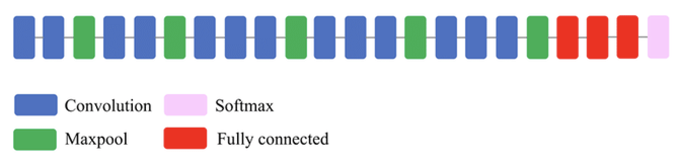
VGG16

• Deeper architecture (16 layers): allows it to learn more complex high-level features
  • Textures, patterns, shapes,...
• Small filters (3x3) work better: capture spatial information while reducing number of parameters
• Max-pooling (2x2): reduces spatial dimension, improves translation invariance
  • Lower resolution forces model to learn robust features (less sensitive to small input changes)
  • Only after every 2 layers, otherwise dimensions reduce too fast
• Downside: too many parameters, expensive to train

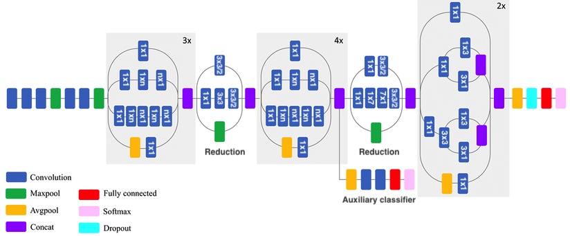
Inceptionv3

• Inception modules: parallel branches learn features of different sizes and scales (3x3, 5x5, 7x7,...)
  • Add reduction blocks that reduce dimensionality via convolutions with stride 2
• Factorized convolutions: a 3x3 conv. can be replaced by combining 1x3 and 3x1, and is 33% cheaper
  • A 5x5 can be replaced by combining 3x3 and 3x3, which can in turn be factorized as above
• 1x1 convolutions, or Network-In-Network (NIN) layers help reduce the number of channels: cheaper
• An auxiliary classifier adds an additional gradient signal deeper in the network

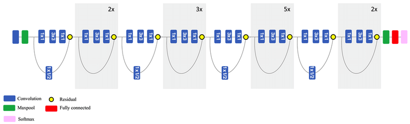
ResNet50

• Residual (skip) connections: add earlier feature map to a later one (dimensions must match)
  • Information can bypass layers, reduces vanishing gradients, allows much deeper nets
• Residual blocks: skip small number or layers and repeat many times
  • Match dimensions though padding and 1x1 convolutions
  • When resolution drops, add 1x1 convolutions with stride 2
• Can be combined with Inception blocks

Interpreting the model

• Let's see what the convnet is learning exactly by observing the intermediate feature maps
  • A layer's output is also called its activation
• We can choose a specific test image, and then retrieve and visualize the activation for every filter for every layer

• Layer 0: has activations of resolution 148x148 for each of its 32 filters
• Layer 2: has activations of resolution 72x72 for each of its 64 filters
• Layer 4: has activations of resolution 34x34 for each of its 128 filters
• Layer 6: has activations of resolution 15x15 for each of its 128 filters

Model: "sequential_3"
_________________________________________________________________
 Layer (type)                Output Shape              Param #   
=================================================================
 conv2d_10 (Conv2D)          (None, 148, 148, 32)      896       
                                                                 
 max_pooling2d_8 (MaxPooling  (None, 74, 74, 32)       0         
 2D)                                                             
                                                                 
 conv2d_11 (Conv2D)          (None, 72, 72, 64)        18496     
                                                                 
 max_pooling2d_9 (MaxPooling  (None, 36, 36, 64)       0         
 2D)                                                             
                                                                 
 conv2d_12 (Conv2D)          (None, 34, 34, 128)       73856     
                                                                 
 max_pooling2d_10 (MaxPoolin  (None, 17, 17, 128)      0         
 g2D)                                                            
                                                                 
 conv2d_13 (Conv2D)          (None, 15, 15, 128)       147584    
                                                                 
 max_pooling2d_11 (MaxPoolin  (None, 7, 7, 128)        0         
 g2D)                                                            
                                                                 
 flatten_2 (Flatten)         (None, 6272)              0         
                                                                 
 dropout (Dropout)           (None, 6272)              0         
                                                                 
 dense_4 (Dense)             (None, 512)               3211776   
                                                                 
 dense_5 (Dense)             (None, 1)                 513       
                                                                 
=================================================================
Total params: 3,453,121
Trainable params: 3,453,121
Non-trainable params: 0
_________________________________________________________________

1/1 [==============================] - 0s 86ms/step

• To extract the activations, we create a new model that outputs the trained layers
  • 8 output layers in total (only the convolutional part)
• We input a test image for prediction and then read the relevant outputs

layer_outputs = [layer.output for layer in model.layers[:8]]
activation_model = models.Model(inputs=model.input, outputs=layer_outputs)
activations = activation_model.predict(img_tensor)

Output of the first Conv2D layer, 3rd channel (filter):

• Similar to a diagonal edge detector
• Your own channels may look different

Output of filter 16:

• Cat eye detector?

The same filter responds quite differently for other inputs (green detector?).

1/1 [==============================] - 0s 9ms/step

• First 2 convolutional layers: various edge detectors

• 3rd convolutional layer: increasingly abstract: ears, eyes

• Last convolutional layer: more abstract patterns
• Empty filter activations: input image does not have the information that the filter was interested in (maybe it was dog-specific)

• Same layer, with dog image input
  • Very different activations

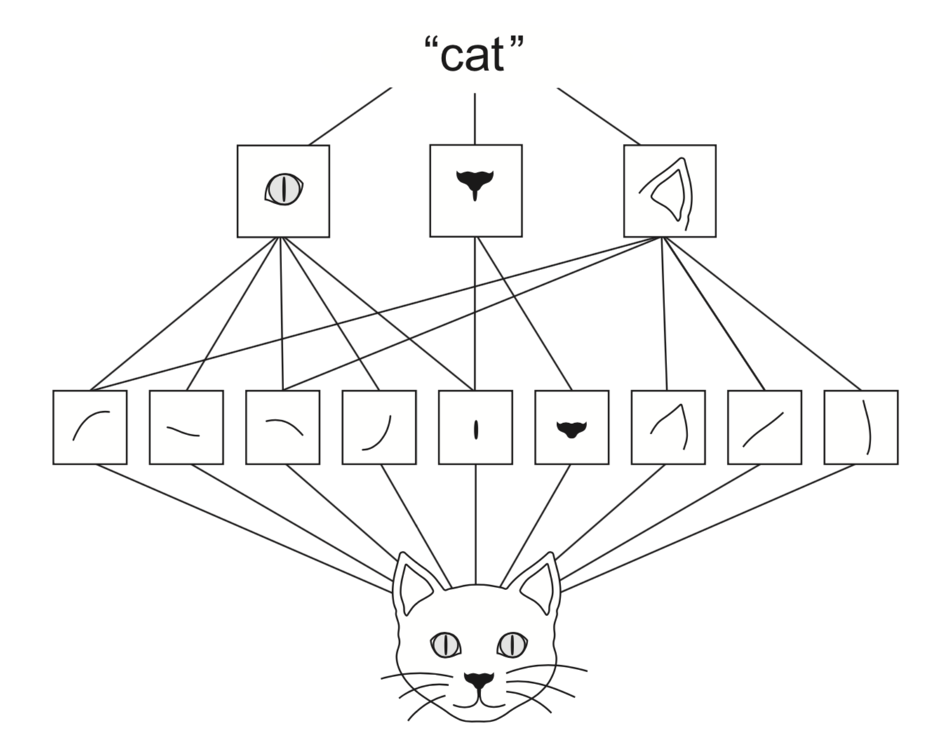
Spatial hierarchies

• Deep convnets can learn spatial hierarchies of patterns
  • First layer can learn very local patterns (e.g. edges)
  • Second layer can learn specific combinations of patterns
  • Every layer can learn increasingly complex abstractions

Visualizing the learned filters

• Visualize filters by finding the input image that they are maximally responsive to
• gradient ascent in input space : start from a random image $x$, use loss to update the input values to values that the filter responds to more strongly (keep weights fixed)
  • $X_{(i+1)} = X_{(i)} + \frac{\partial L(x, X_{(i)})}{\partial X} * \eta$

from keras import backend as K
    input_img = np.random.random((1, size, size, 3)) * 20 + 128.
    loss = K.mean(layer_output[:, :, :, filter_index])
    grads = K.gradients(loss, model.input)[0] # Compute gradient
    for i in range(40): # Run gradient ascent for 40 steps
        loss_v, grads_v = K.function([input_img], [loss, grads])
        input_img_data += grads_v * step

• Learned filters of last convolutional layer
• More focused on center, some vague cat/dog head shapes

Let's do this again for the VGG16 network pretrained on ImageNet (much larger)

model = VGG16(weights='imagenet', include_top=False)

Model: "vgg16"
_________________________________________________________________
 Layer (type)                Output Shape              Param #   
=================================================================
 input_1 (InputLayer)        [(None, None, None, 3)]   0         
                                                                 
 block1_conv1 (Conv2D)       (None, None, None, 64)    1792      
                                                                 
 block1_conv2 (Conv2D)       (None, None, None, 64)    36928     
                                                                 
 block1_pool (MaxPooling2D)  (None, None, None, 64)    0         
                                                                 
 block2_conv1 (Conv2D)       (None, None, None, 128)   73856     
                                                                 
 block2_conv2 (Conv2D)       (None, None, None, 128)   147584    
                                                                 
 block2_pool (MaxPooling2D)  (None, None, None, 128)   0         
                                                                 
 block3_conv1 (Conv2D)       (None, None, None, 256)   295168    
                                                                 
 block3_conv2 (Conv2D)       (None, None, None, 256)   590080    
                                                                 
 block3_conv3 (Conv2D)       (None, None, None, 256)   590080    
                                                                 
 block3_pool (MaxPooling2D)  (None, None, None, 256)   0         
                                                                 
 block4_conv1 (Conv2D)       (None, None, None, 512)   1180160   
                                                                 
 block4_conv2 (Conv2D)       (None, None, None, 512)   2359808   
                                                                 
 block4_conv3 (Conv2D)       (None, None, None, 512)   2359808   
                                                                 
 block4_pool (MaxPooling2D)  (None, None, None, 512)   0         
                                                                 
 block5_conv1 (Conv2D)       (None, None, None, 512)   2359808   
                                                                 
 block5_conv2 (Conv2D)       (None, None, None, 512)   2359808   
                                                                 
 block5_conv3 (Conv2D)       (None, None, None, 512)   2359808   
                                                                 
 block5_pool (MaxPooling2D)  (None, None, None, 512)   0         
                                                                 
=================================================================
Total params: 14,714,688
Trainable params: 14,714,688
Non-trainable params: 0
_________________________________________________________________

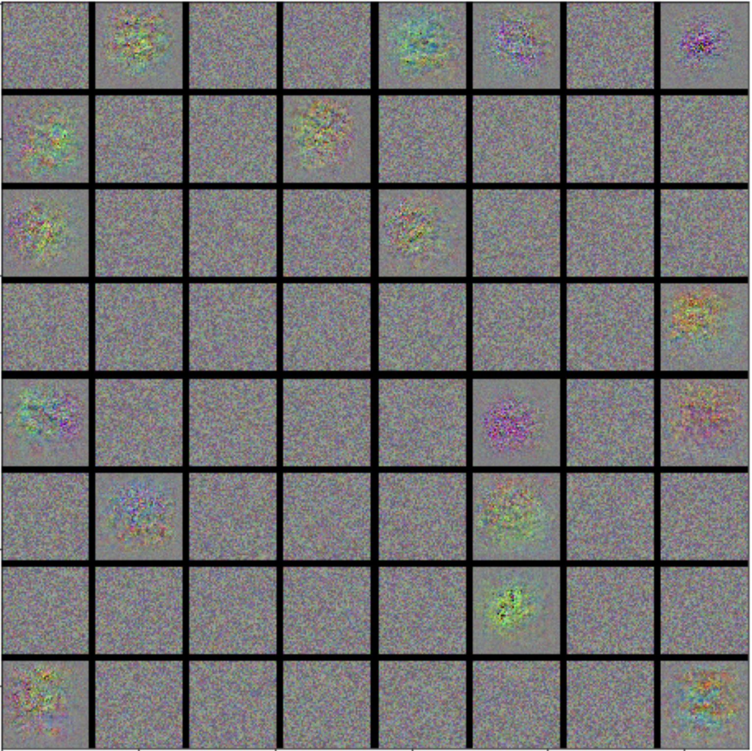
• Visualize convolution filters 0-2 from layer 5 of the VGG network trained on ImageNet
• Some respond to dots or waves in the image

First 64 filters for 1st convolutional layer in block 1: simple edges and colors

Filters in 2nd block of convolution layers: simple textures (combined edges and colors)

Filters in 3rd block of convolution layers: more natural textures

Filters in 4th block of convolution layers: feathers, eyes, leaves,...

Visualizing class activation

• We can also visualize which part of the input image had the greatest influence on the final classification. Helps to interpret what the model is paying attention to.
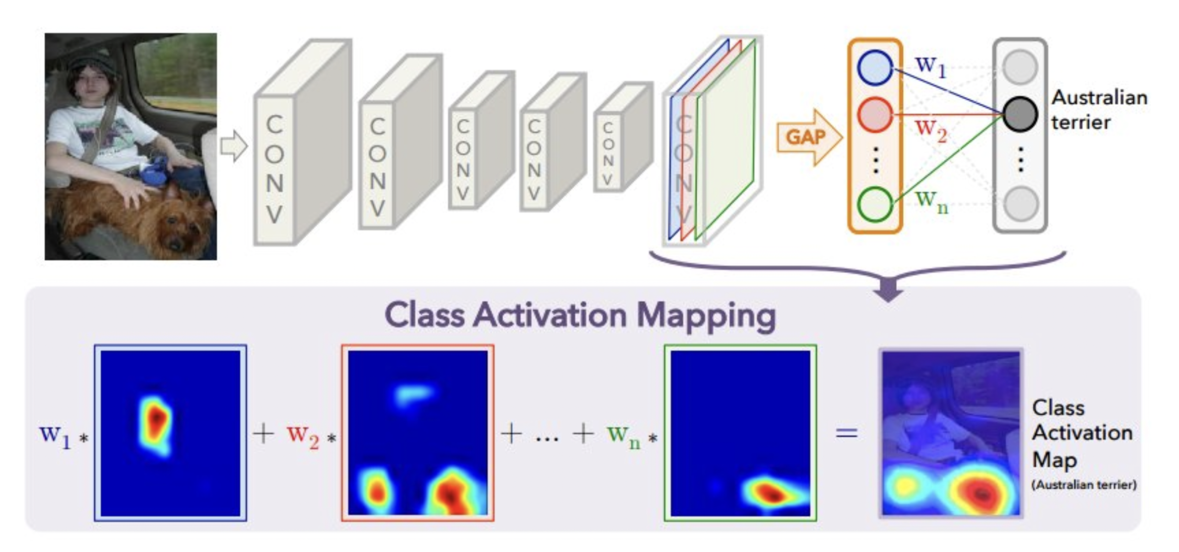
• Class activation maps : produces a heatmap over the input image
  • Choose a convolution layer, do Global Average Pooling (GAP) to get one output per filter
  • Get the weights between those outputs and the class of interest
  • Compute the weighted sum of all filter activations: combines what each filter is responding to and how much this affects the class prediction

Example on VGG with a specific input image

• Take the last convolutional layer of VGG pretrained on ImageNet
  • It consists of 512 filters of size 14x14

model = VGG16(weights='imagenet')
last_conv_layer = model.get_layer('block5_conv3')

Last conv layer shape: (None, 14, 14, 512)

• Choose an input image and preprocess it so we can feed it to the model

img = image.load_img(img_path, target_size=(224, 224))

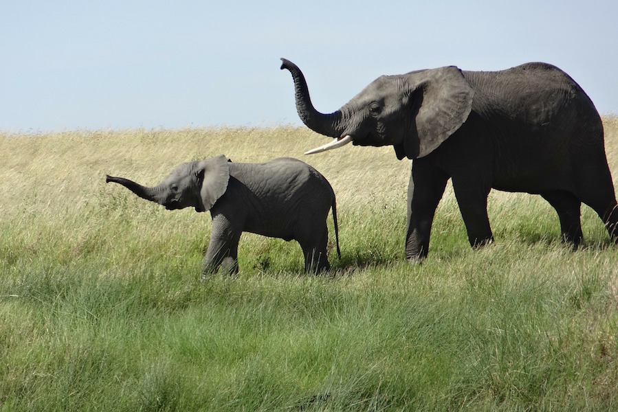
• Find the output node for its class ('african elephant', class 386)

african_elephant_output = model.output[:, 386]

• VGG doesn't use GAP. Compute the average gradient from the output node to the conv layer
• Multiply (channel-wise) with the activations of the conv layer

grads = K.gradients(african_elephant_output, last_conv_layer.output)[0]
pooled_grads = K.mean(grads, axis=(0, 1, 2))
for i in range(512): # 512 filters
    conv_layer_output_value[:, :, i] *= pooled_grads_value[i]
heatmap = np.mean(conv_layer_output_value, axis=-1)

• Visualize heatmap. It's 14x14 since that's the output dimension of the conv layer

• Upscaled and superimposed on the original image
• The model looked at the face of the baby elephant and the trunk of the large elephant

Transfer learning

• We can re-use pretrained networks instead of training from scratch
• Learned features can be a generic model of the visual world
• Use convolutional base to contruct features, then train any classifier on new data
• Also called transfer learning , which is a kind of meta-learning

• Let's instantiate the VGG16 model (without the dense layers)
• With 150x150 inputs, the final feature map has shape (4, 4, 512)

conv_base = VGG16(weights='imagenet', include_top=False, input_shape=(150, 150, 3))

Model: "vgg16"
_________________________________________________________________
 Layer (type)                Output Shape              Param #   
=================================================================
 input_2 (InputLayer)        [(None, 150, 150, 3)]     0         
                                                                 
 block1_conv1 (Conv2D)       (None, 150, 150, 64)      1792      
                                                                 
 block1_conv2 (Conv2D)       (None, 150, 150, 64)      36928     
                                                                 
 block1_pool (MaxPooling2D)  (None, 75, 75, 64)        0         
                                                                 
 block2_conv1 (Conv2D)       (None, 75, 75, 128)       73856     
                                                                 
 block2_conv2 (Conv2D)       (None, 75, 75, 128)       147584    
                                                                 
 block2_pool (MaxPooling2D)  (None, 37, 37, 128)       0         
                                                                 
 block3_conv1 (Conv2D)       (None, 37, 37, 256)       295168    
                                                                 
 block3_conv2 (Conv2D)       (None, 37, 37, 256)       590080    
                                                                 
 block3_conv3 (Conv2D)       (None, 37, 37, 256)       590080    
                                                                 
 block3_pool (MaxPooling2D)  (None, 18, 18, 256)       0         
                                                                 
 block4_conv1 (Conv2D)       (None, 18, 18, 512)       1180160   
                                                                 
 block4_conv2 (Conv2D)       (None, 18, 18, 512)       2359808   
                                                                 
 block4_conv3 (Conv2D)       (None, 18, 18, 512)       2359808   
                                                                 
 block4_pool (MaxPooling2D)  (None, 9, 9, 512)         0         
                                                                 
 block5_conv1 (Conv2D)       (None, 9, 9, 512)         2359808   
                                                                 
 block5_conv2 (Conv2D)       (None, 9, 9, 512)         2359808   
                                                                 
 block5_conv3 (Conv2D)       (None, 9, 9, 512)         2359808   
                                                                 
 block5_pool (MaxPooling2D)  (None, 4, 4, 512)         0         
                                                                 
=================================================================
Total params: 14,714,688
Trainable params: 14,714,688
Non-trainable params: 0
_________________________________________________________________

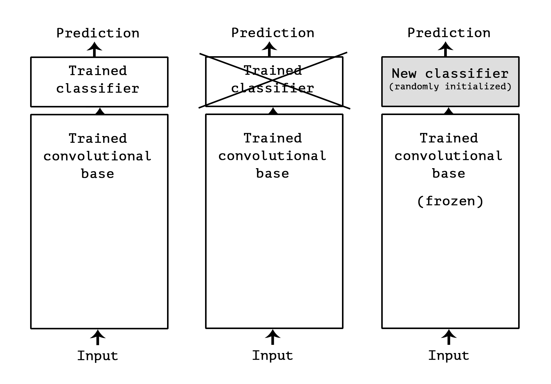
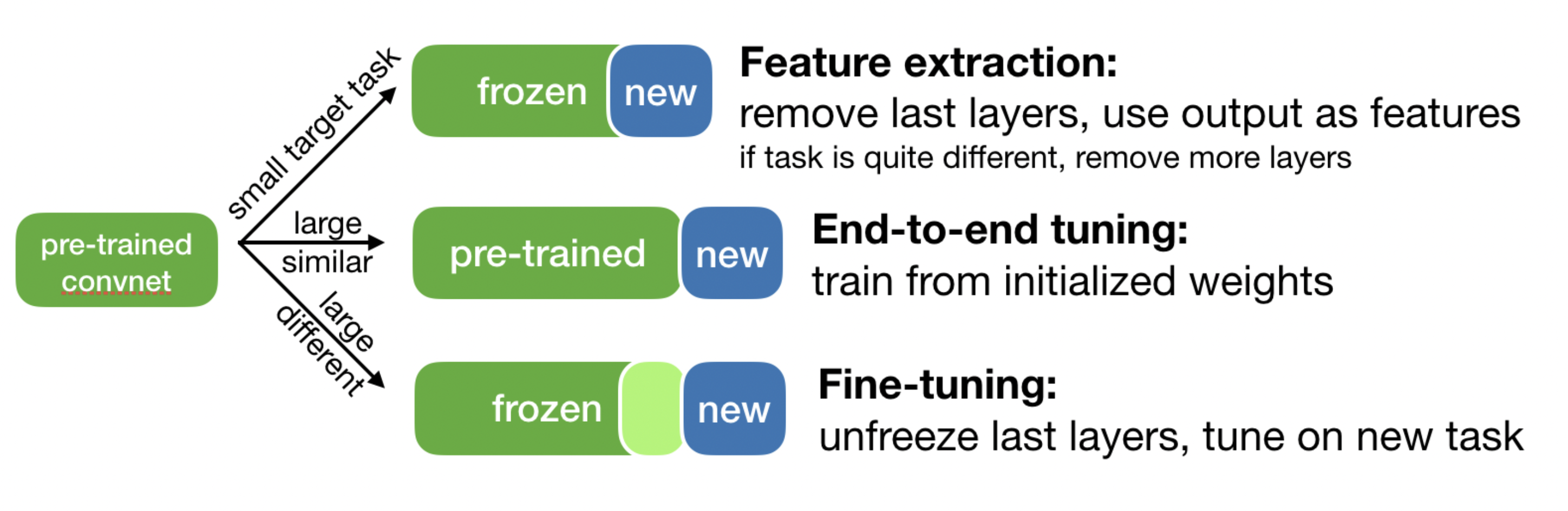
Using pre-trained networks: 3 ways

• Fast feature extraction (for similar task, little data)
  • Call predict from the convolutional base to build new features
  • Use outputs as input to a new neural net (or other algorithm)
• End-to-end tuning (for similar task, lots of data + data augmentation)
  • Extend the convolutional base model with a new dense layer
  • Train it end to end on the new data (expensive!)
• Fine-tuning (for somewhat different task)
  • Unfreeze a few of the top convolutional layers, and retrain
  • Update only the more abstract representations

Fast feature extraction (without data augmentation)

• Run every batch through the pre-trained convolutional base

features = conv_base.predict(inputs)

• Build Dense neural net (with Dropout)
• Train and evaluate with the transformed examples

model = models.Sequential()
model.add(layers.Dense(256, activation='relu', input_dim=4 * 4 * 512))
model.add(layers.Dropout(0.5))
model.add(layers.Dense(1, activation='sigmoid'))

model.fit(features, labels, epochs=30)

• Validation accuracy around 90%, much better!
• Still overfitting, despite the Dropout: not enough training data

Max val_acc 0.90500003

Fast feature extraction (with data augmentation)

• Simply add the Dense layers to the convolutional base
• Freeze the convolutional base (before you compile)
  • Without freezing, you train it end-to-end (expensive)

model = models.Sequential()
model.add(conv_base)
model.add(layers.Flatten())
model.add(layers.Dense(256, activation='relu'))
model.add(layers.Dense(1, activation='sigmoid'))
conv_base.trainable = False # Freeze the pretrained weights

We now get about 90% accuracy again, and very little overfitting

Max val_acc 0.906

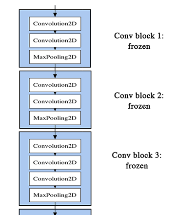
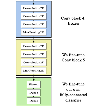
Fine-tuning

• Add your custom network on top of an already trained base network.
• Freeze the base network, but unfreeze the last block of conv layers.

for layer in conv_base.layers:
    if layer.name == 'block5_conv1':
        layer.trainable = True
    else:
        layer.trainable = False

Visualized

• Load trained network, finetune
  • Use a small learning rate, large number of epochs
  • You don't want to unlearn too much: catastrophic forgetting

model = load_model(os.path.join(model_dir, 'cats_and_dogs_small_3b.h5'))
model.compile(loss='binary_crossentropy', 
              optimizer=optimizers.RMSprop(lr=1e-5),
              metrics=['acc'])
history = model.fit(
      train_generator, steps_per_epoch=100, epochs=100,
      validation_data=validation_generator,
      validation_steps=50)

Almost 95% accuracy. The curves are quite noisy, though.

Max val_acc 0.90800005

• We can smooth the learning curves using a running average

Max val_acc 0.9039536851123335

Take-aways

• Convnets are ideal for addressing image-related problems.
• They learn a hierarchy of modular patterns and concepts to represent the visual world.
• Representations are easy to inspect
• Data augmentation helps fight overfitting
• You can use a pretrained convnet to build better models via transfer learning