Lecture 7: Convolutional Neural Networks

Handling image data

Joaquin Vanschoren, Eindhoven University of Technology

Overview

• Image convolution
• Convolutional neural networks
• Data augmentation
• Real-world CNNs
• Model interpretation
• Using pre-trained networks (transfer learning)

Convolutions

• Operation that transforms an image by sliding a smaller image (called a filter or kernel ) over the image and multiplying the pixel values
  • Slide an $n$ x $n$ filter over $n$ x $n$ patches of the original image
  • Every pixel is replaced by the sum of the element-wise products of the values of the image patch around that pixel and the kernel

# kernel and image_patch are n x n matrices
pixel_out = np.sum(kernel * image_patch)

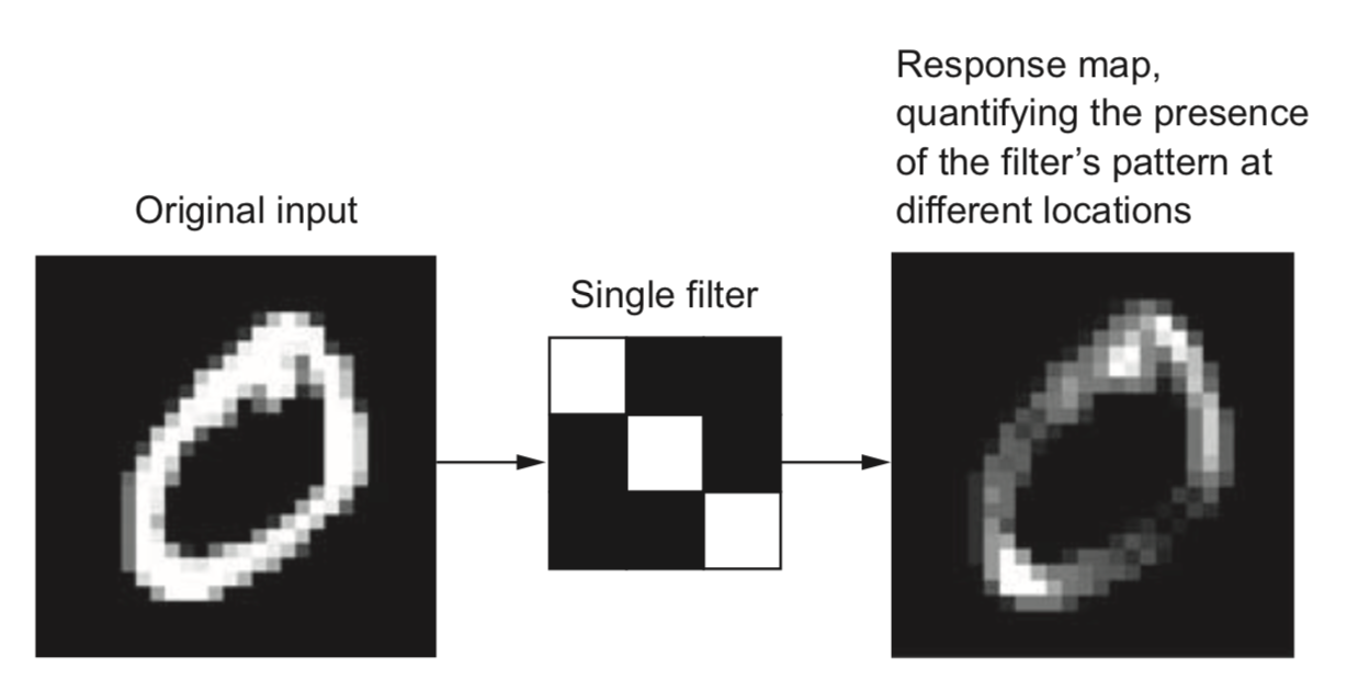
• Different kernels can detect different types of patterns in the image

Demonstration on Fashion-MNIST

Demonstration of convolution with edge filters

Image convolution in practice

• How do we know which filters are best for a given image?
• Families of kernels (or filter banks ) can be run on every image
  • Gabor, Sobel, Haar Wavelets,...
• Gabor filters: Wave patterns generated by changing:
  • Frequency: narrow or wide ondulations
  • Theta: angle (direction) of the wave
  • Sigma: resolution (size of the filter)

Demonstration of Gabor filters

Demonstration on the Fashion-MNIST data

Filter banks

• Different filters detect different edges, shapes,...
• Not all seem useful

Convolutional neural nets

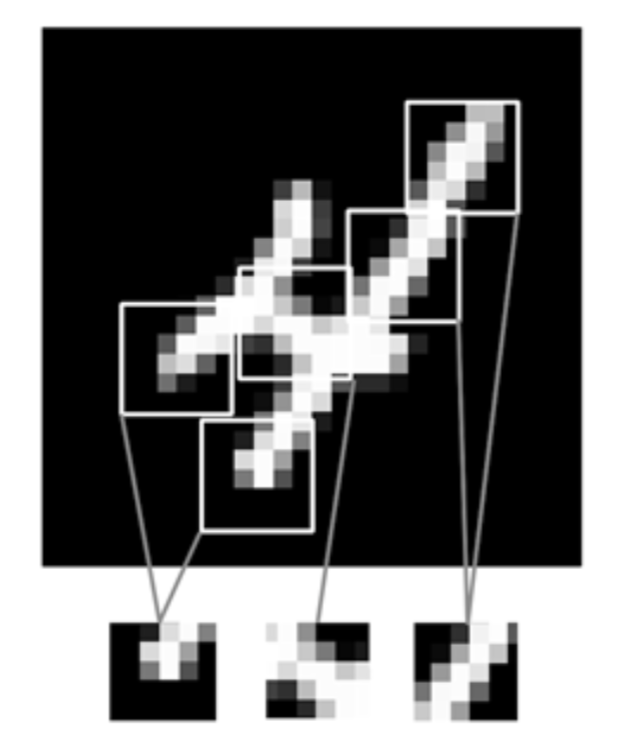
• Finding relationships between individual pixels and the correct class is hard
• Simplify the problem by decomposing it into smaller problems
• First, discover 'local' patterns (edges, lines, endpoints)
• Representing such local patterns as features makes it easier to learn from them
  • Deeper layers will do that for us
• We could use convolutions, but how to choose the filters?

Convolutional Neural Networks (ConvNets)

• Instead of manually designing the filters, we can also learn them based on data
  • Choose filter sizes (manually), initialize with small random weights
• Forward pass: Convolutional layer slides the filter over the input, generates the output
• Backward pass: Update the filter weights according to the loss gradients
• Illustration for 1 filter:

Convolutional layers: Feature maps

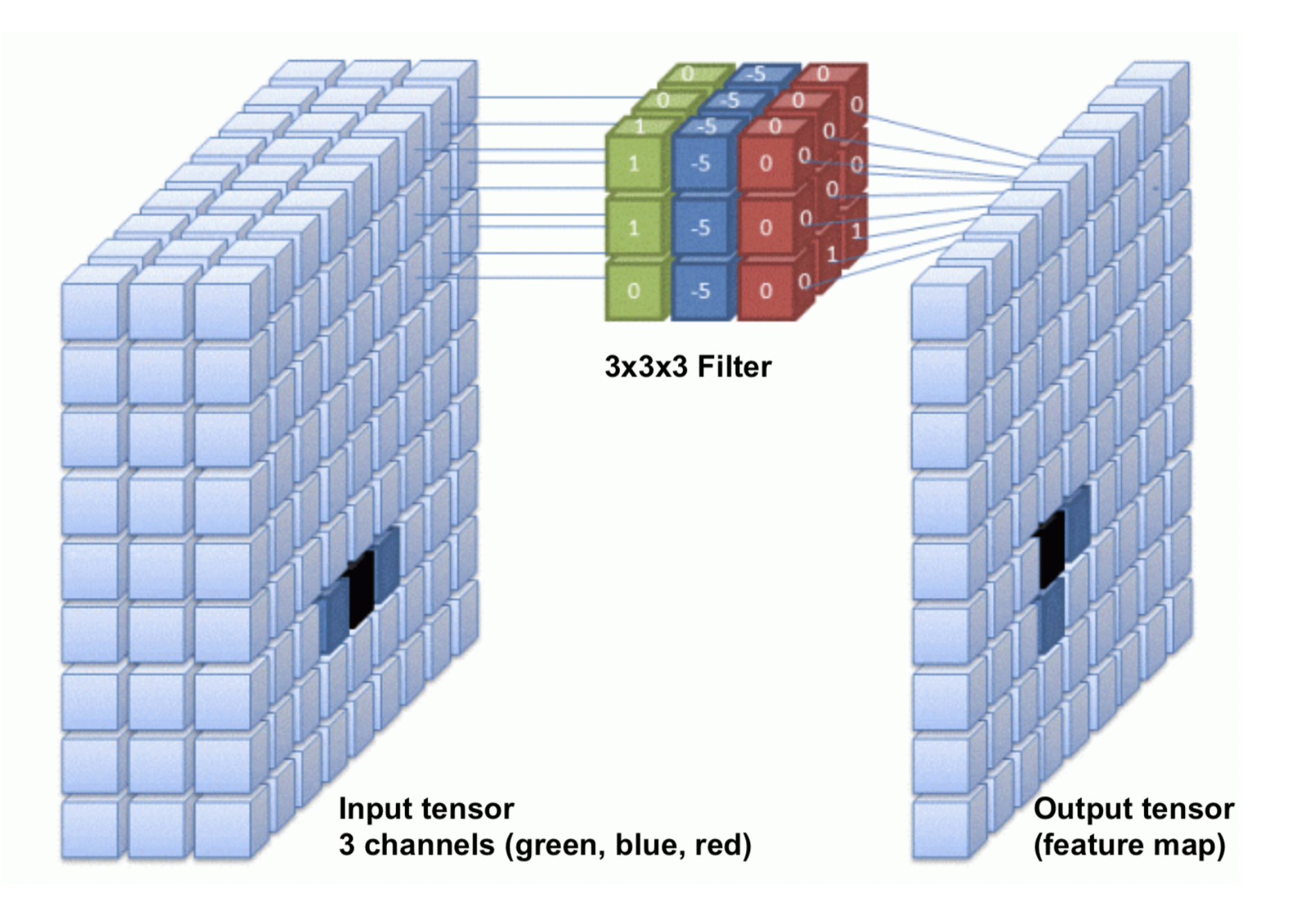
• One filter is not sufficient to detect all relevant patterns in an image
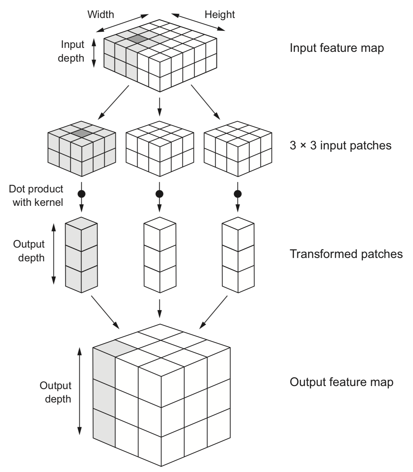
• A convolutional layer applies and learns $d$ filters in parallel
• Slide $d$ filters across the input image (in parallel) -> a (1x1xd) output per patch
• Reassemble into a feature map with $d$ 'channels', a (width x height x d) tensor.

Border effects (zero padding)

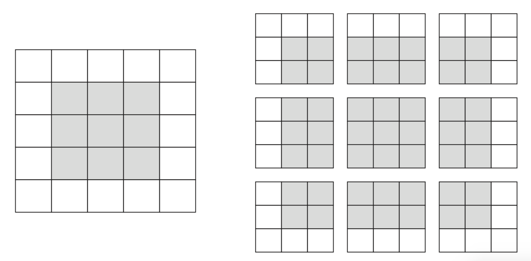
• Consider a 5x5 image and a 3x3 filter: there are only 9 possible locations, hence the output is a 3x3 feature map
• If we want to maintain the image size, we use zero-padding, adding 0's all around the input tensor.

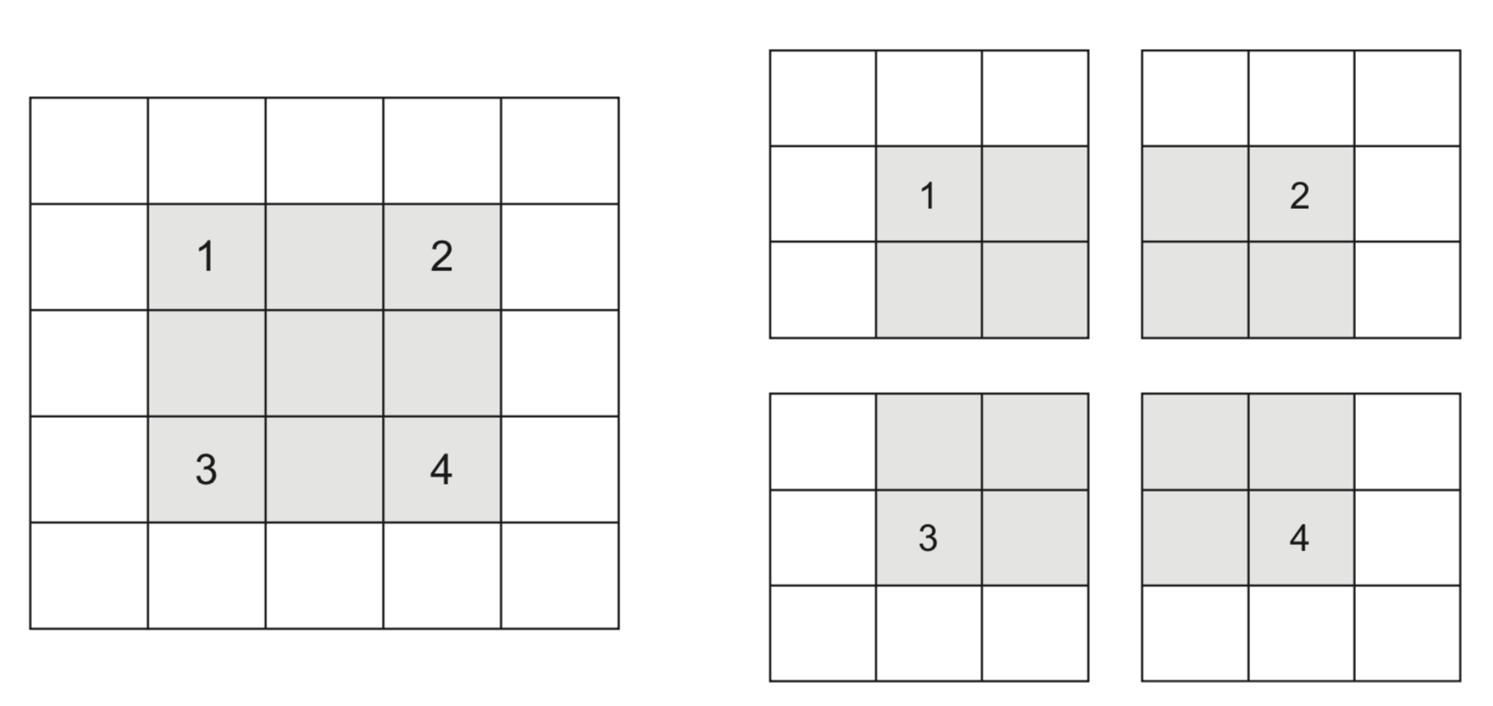
Undersampling (striding)

• Sometimes, we want to downsample a high-resolution image
  • Faster processing, less noisy (hence less overfitting)
  • Forces the model to summarize information in (smaller) feature maps
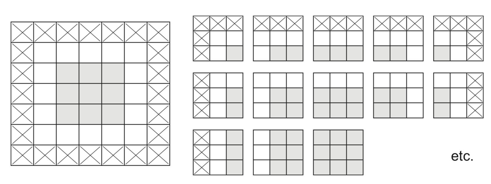
• One approach is to skip values during the convolution
  • Distance between 2 windows: stride length
• Example with stride length 2 (without padding):

Max-pooling

• Another approach to shrink the input tensors is max-pooling :
  • Run a filter with a fixed stride length over the image
    • Usually 2x2 filters and stride lenght 2
  • The filter simply returns the max (or avg ) of all values
• Agressively reduces the number of weights (less overfitting)

Receptive field

• Receptive field: how much each output neuron 'sees' of the input image
• Translation invariance: shifting the input does not affect the output
  • Large receptive field -> neurons can 'see' patterns anywhere in the input
• $nxn$ convolutions only increase the receptive field by $n+2$ each layer
• Maxpooling doubles the receptive field without deepening the network

Dilated convolutions

• Downsample by introducing 'gaps' between filter elements by spacing them out
• Increases the receptive field exponentially
• Doesn't need extra parameters or computation (unlike larger filters)
• Retains feature map size (unlike pooling)

Convolutional nets in practice

• Use multiple convolutional layers to learn patterns at different levels of abstraction
  • Find local patterns first (e.g. edges), then patterns across those patterns
• Use MaxPooling layers to reduce resolution, increase translation invariance
• Use sufficient filters in the first layer (otherwise information gets lost)
• In deeper layers, use increasingly more filters
  • Preserve information about the input as resolution descreases
  • Avoid decreasing the number of activations (resolution x nr of filters)
• For very deep nets, add skip connections to preserve information (and gradients)
  • Sums up outputs of earlier layers to those of later layers (with same dimensions)

Example with PyTorch

• Conv2d for 2D convolutional layers
  • Grayscale image: 1 in_channels
  • 32 filters: 32 out_channels, 3x3 size
  • Deeper layers use 64 filters
  • ReLU activation, no padding
  • MaxPool2d for max-pooling, 2x2

model = nn.Sequential(
    nn.Conv2d(in_channels=1, out_channels=32, kernel_size=3),
    nn.ReLU(),
    nn.MaxPool2d(kernel_size=2, stride=2),
    nn.Conv2d(in_channels=32, out_channels=64, kernel_size=3),
    nn.ReLU(),
    nn.MaxPool2d(kernel_size=2, stride=2),
    nn.Conv2d(in_channels=64, out_channels=64, kernel_size=3),
    nn.ReLU()
)

• Observe how the input image on 1x28x28 is transformed to a 64x3x3 feature map
  • In pytorch, shapes are (batch_size, channels, height, width)
• Conv2d parameters = (kernel size^2 × input channels + 1) × output channels
• No zero-padding: every output is 2 pixels less in every dimension
• After every MaxPooling, resolution halved in every dimension

==========================================================================================
Layer (type:depth-idx)                   Output Shape              Param #
==========================================================================================
Sequential                               [1, 64, 3, 3]             --
├─Conv2d: 1-1                            [1, 32, 26, 26]           320
├─ReLU: 1-2                              [1, 32, 26, 26]           --
├─MaxPool2d: 1-3                         [1, 32, 13, 13]           --
├─Conv2d: 1-4                            [1, 64, 11, 11]           18,496
├─ReLU: 1-5                              [1, 64, 11, 11]           --
├─MaxPool2d: 1-6                         [1, 64, 5, 5]             --
├─Conv2d: 1-7                            [1, 64, 3, 3]             36,928
├─ReLU: 1-8                              [1, 64, 3, 3]             --
==========================================================================================
Total params: 55,744
Trainable params: 55,744
Non-trainable params: 0
Total mult-adds (M): 2.79
==========================================================================================
Input size (MB): 0.00
Forward/backward pass size (MB): 0.24
Params size (MB): 0.22
Estimated Total Size (MB): 0.47
==========================================================================================

• To classify the images, we still need a linear and output layer.
• We flatten the 3x3x64 feature map to a vector of size 576

model = nn.Sequential(
    ...
    nn.Conv2d(in_channels=64, out_channels=64, kernel_size=3, padding=0),
    nn.ReLU(),
    nn.Flatten(),
    nn.Linear(64 * 3 * 3, 64),
    nn.ReLU(),
    nn.Linear(64, 10)
)

Complete model. Flattening adds a lot of weights!

==========================================================================================
Layer (type:depth-idx)                   Output Shape              Param #
==========================================================================================
Sequential                               [1, 10]                   --
├─Conv2d: 1-1                            [1, 32, 26, 26]           320
├─ReLU: 1-2                              [1, 32, 26, 26]           --
├─MaxPool2d: 1-3                         [1, 32, 13, 13]           --
├─Conv2d: 1-4                            [1, 64, 11, 11]           18,496
├─ReLU: 1-5                              [1, 64, 11, 11]           --
├─MaxPool2d: 1-6                         [1, 64, 5, 5]             --
├─Conv2d: 1-7                            [1, 64, 3, 3]             36,928
├─ReLU: 1-8                              [1, 64, 3, 3]             --
├─Flatten: 1-9                           [1, 576]                  --
├─Linear: 1-10                           [1, 64]                   36,928
├─ReLU: 1-11                             [1, 64]                   --
├─Linear: 1-12                           [1, 10]                   650
==========================================================================================
Total params: 93,322
Trainable params: 93,322
Non-trainable params: 0
Total mult-adds (M): 2.82
==========================================================================================
Input size (MB): 0.00
Forward/backward pass size (MB): 0.24
Params size (MB): 0.37
Estimated Total Size (MB): 0.62
==========================================================================================

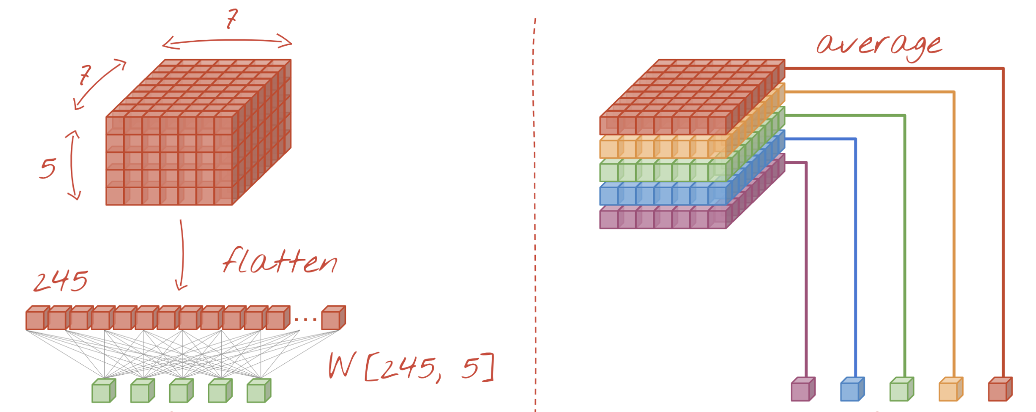
Global Average Pooling (GAP)

• Instead of flattening, we do GAP: returns average of each activation map
• We can drop the hidden dense layer: number of outputs > number of classes

model = nn.Sequential(...
    nn.AdaptiveAvgPool2d(1), # Global Average Pooling
    nn.Flatten(),            # Convert (batch, 64, 1, 1) -> (batch, 64)
    nn.Linear(64, 10))       # Output layer for 10 classes

• With GlobalAveragePooling: much fewer weights to learn
• Use with caution: this destroys the location information learned by the CNN
• Not ideal for tasks such as object localization

==========================================================================================
Layer (type:depth-idx)                   Output Shape              Param #
==========================================================================================
Sequential                               [1, 10]                   --
├─Conv2d: 1-1                            [1, 32, 26, 26]           320
├─ReLU: 1-2                              [1, 32, 26, 26]           --
├─MaxPool2d: 1-3                         [1, 32, 13, 13]           --
├─Conv2d: 1-4                            [1, 64, 11, 11]           18,496
├─ReLU: 1-5                              [1, 64, 11, 11]           --
├─MaxPool2d: 1-6                         [1, 64, 5, 5]             --
├─Conv2d: 1-7                            [1, 64, 3, 3]             36,928
├─ReLU: 1-8                              [1, 64, 3, 3]             --
├─AdaptiveAvgPool2d: 1-9                 [1, 64, 1, 1]             --
├─Flatten: 1-10                          [1, 64]                   --
├─Linear: 1-11                           [1, 10]                   650
==========================================================================================
Total params: 56,394
Trainable params: 56,394
Non-trainable params: 0
Total mult-adds (M): 2.79
==========================================================================================
Input size (MB): 0.00
Forward/backward pass size (MB): 0.24
Params size (MB): 0.23
Estimated Total Size (MB): 0.47
==========================================================================================

Run the model on MNIST dataset

• Train and test as usual: 99% accuracy
  • Compared to 97,8% accuracy with the dense architecture
  • Flatten and GlobalAveragePooling yield similar performance

Cats vs Dogs

• A more realistic dataset: Cats vs Dogs
  • Colored JPEG images, different sizes
  • Not nicely centered, translation invariance is important
• Preprocessing
  • Decode JPEG images to floating-point tensors
  • Rescale pixel values to [0,1]
  • Resize images to 150x150 pixels

Data loader

• We create a Pytorch Lightning DataModule to do preprocessing and data loading

class ImageDataModule(pl.LightningDataModule):
  def __init__(self, data_dir, batch_size=20, img_size=(150, 150)):
    super().__init__()
    self.transform = transforms.Compose([
      transforms.Resize(self.img_size),  # Resize to 150x150
      transforms.ToTensor()])  # Convert to tensor (also scales 0-1)
  def setup(self, stage=None):
    self.train_dataset = datasets.ImageFolder(root=train_dir, transform=self.transform)
    self.val_dataset = datasets.ImageFolder(root=val_dir, transform=self.transform)

  def train_dataloader(self):
    return DataLoader(self.train_dataset, batch_size=self.batch_size, shuffle=True)
  def val_dataloader(self):
    return DataLoader(self.val_dataset, batch_size=self.batch_size, shuffle=False)

Model

Since the images are more complex, we add another convolutional layer and increase the number of filters to 128.

==========================================================================================
Layer (type:depth-idx)                   Output Shape              Param #
==========================================================================================
CatImageClassifier                       [1, 1]                    --
├─Sequential: 1-1                        [1, 128, 1, 1]            --
│    └─Conv2d: 2-1                       [1, 32, 148, 148]         896
│    └─ReLU: 2-2                         [1, 32, 148, 148]         --
│    └─MaxPool2d: 2-3                    [1, 32, 74, 74]           --
│    └─Conv2d: 2-4                       [1, 64, 72, 72]           18,496
│    └─ReLU: 2-5                         [1, 64, 72, 72]           --
│    └─MaxPool2d: 2-6                    [1, 64, 36, 36]           --
│    └─Conv2d: 2-7                       [1, 128, 34, 34]          73,856
│    └─ReLU: 2-8                         [1, 128, 34, 34]          --
│    └─MaxPool2d: 2-9                    [1, 128, 17, 17]          --
│    └─Conv2d: 2-10                      [1, 128, 15, 15]          147,584
│    └─ReLU: 2-11                        [1, 128, 15, 15]          --
│    └─MaxPool2d: 2-12                   [1, 128, 7, 7]            --
│    └─AdaptiveAvgPool2d: 2-13           [1, 128, 1, 1]            --
├─Sequential: 1-2                        [1, 1]                    --
│    └─Linear: 2-14                      [1, 512]                  66,048
│    └─ReLU: 2-15                        [1, 512]                  --
│    └─Linear: 2-16                      [1, 1]                    513
==========================================================================================
Total params: 307,393
Trainable params: 307,393
Non-trainable params: 0
Total mult-adds (M): 234.16
==========================================================================================
Input size (MB): 0.27
Forward/backward pass size (MB): 9.68
Params size (MB): 1.23
Estimated Total Size (MB): 11.18
==========================================================================================

Training

• We use a Trainer module (from PyTorch Lightning) to simplify training

trainer = pl.Trainer(
    max_epochs=20,        # Train for 20 epochs
    accelerator="gpu",    # Move data and model to GPU
    devices="auto",       # Number of GPUs
    deterministic=True,   # Set random seeds, for reproducibility
    callbacks=[metric_tracker,      # Callback for logging loss and acc
               checkpoint_callback] # Callback for logging weights
)
trainer.fit(model, datamodule=data_module)

• Tip: to store the best model weights, you can add a ModelCheckpoint callback

checkpoint_callback = ModelCheckpoint(
    monitor="val_loss",   # Save model with lowest val. loss
    mode="min",           # "min" for loss, "max" for accuracy
    save_top_k=1,         # Keep only the best model
    dirpath="weights/",   # Directory to save checkpoints
    filename="cat_model", # File name pattern
)

The model learns well for the first 20 epochs, but then starts overfitting a lot!

Solving overfitting in CNNs

• There are various ways to further improve the model:
  • Generating more training data (data augmentation)
  • Regularization (e.g. Dropout, L1/L2, Batch Normalization,...)
  • Use pretrained rather than randomly initialized filters
    • These are trained on a lot more data

Data augmentation

• Generate new images via image transformations (only on training data!)
  • Images will be randomly transformed every epoch
• Update the transform in the data module

self.train_transform = transforms.Compose([
    transforms.Resize(self.img_size), # Resize to 150x150
    transforms.RandomRotation(40),    # Rotations up to 40 degrees
    transforms.RandomResizedCrop(self.img_size, 
                                 scale=(0.8, 1.2)), # Scale + crop, up to 20%
    transforms.RandomHorizontalFlip(),              # Horizontal flip
    transforms.RandomAffine(degrees=0, shear=20),   # Shear, up to 20%
    transforms.ColorJitter(brightness=0.2, contrast=0.2, 
                           saturation=0.2),         # Color jitter

    transforms.ToTensor(),
    transforms.Normalize(mean=[0.5, 0.5, 0.5], std=[0.5, 0.5, 0.5])
    ])

Augmentation example

We also add Dropout before the Dense layer, and L2 regularization ('weight decay') in Adam

==========================================================================================
Layer (type:depth-idx)                   Output Shape              Param #
==========================================================================================
CatImageClassifier                       [1, 1]                    --
├─Sequential: 1-1                        [1, 128, 1, 1]            --
│    └─Conv2d: 2-1                       [1, 32, 148, 148]         896
│    └─ReLU: 2-2                         [1, 32, 148, 148]         --
│    └─MaxPool2d: 2-3                    [1, 32, 74, 74]           --
│    └─Conv2d: 2-4                       [1, 64, 72, 72]           18,496
│    └─ReLU: 2-5                         [1, 64, 72, 72]           --
│    └─MaxPool2d: 2-6                    [1, 64, 36, 36]           --
│    └─Conv2d: 2-7                       [1, 128, 34, 34]          73,856
│    └─ReLU: 2-8                         [1, 128, 34, 34]          --
│    └─MaxPool2d: 2-9                    [1, 128, 17, 17]          --
│    └─Conv2d: 2-10                      [1, 128, 15, 15]          147,584
│    └─ReLU: 2-11                        [1, 128, 15, 15]          --
│    └─MaxPool2d: 2-12                   [1, 128, 7, 7]            --
│    └─AdaptiveAvgPool2d: 2-13           [1, 128, 1, 1]            --
├─Sequential: 1-2                        [1, 1]                    --
│    └─Linear: 2-14                      [1, 512]                  66,048
│    └─ReLU: 2-15                        [1, 512]                  --
│    └─Dropout: 2-16                     [1, 512]                  --
│    └─Linear: 2-17                      [1, 1]                    513
==========================================================================================
Total params: 307,393
Trainable params: 307,393
Non-trainable params: 0
Total mult-adds (M): 234.16
==========================================================================================
Input size (MB): 0.27
Forward/backward pass size (MB): 9.68
Params size (MB): 1.23
Estimated Total Size (MB): 11.18
==========================================================================================

No more overfitting!

Real-world CNNs

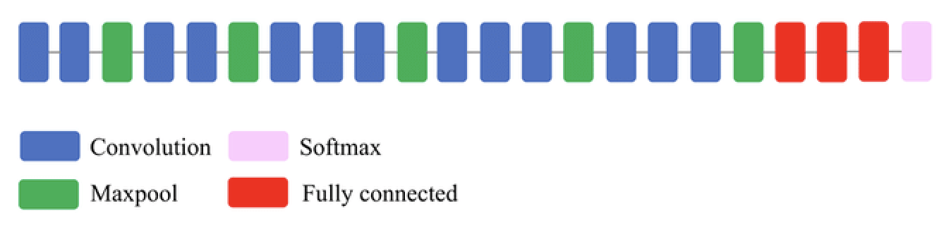
VGG16

• Deeper architecture (16 layers): allows it to learn more complex high-level features
  • Textures, patterns, shapes,...
• Small filters (3x3) work better: capture spatial information while reducing number of parameters
• Max-pooling (2x2): reduces spatial dimension, improves translation invariance
  • Lower resolution forces model to learn robust features (less sensitive to small input changes)
  • Only after every 2 layers, otherwise dimensions reduce too fast
• Downside: too many parameters, expensive to train

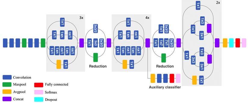
Inceptionv3

• Inception modules: parallel branches learn features of different sizes and scales (3x3, 5x5, 7x7,...)
  • Add reduction blocks that reduce dimensionality via convolutions with stride 2
• Factorized convolutions: a 3x3 conv. can be replaced by combining 1x3 and 3x1, and is 33% cheaper
  • A 5x5 can be replaced by combining 3x3 and 3x3, which can in turn be factorized as above
• 1x1 convolutions, or Network-In-Network (NIN) layers help reduce the number of channels: cheaper
• An auxiliary classifier adds an additional gradient signal deeper in the network

Factorized convolutions

• A 3x3 conv. can be replaced by combining 1x3 and 3x1, and is 33% cheaper

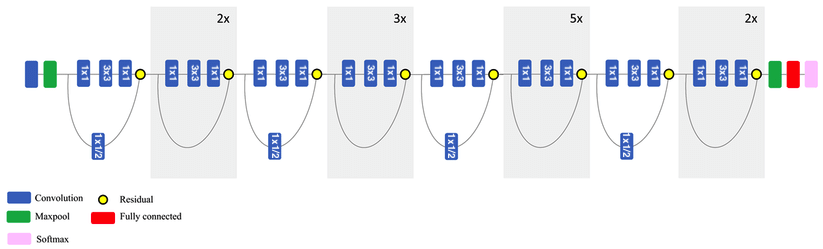
ResNet50

• Residual (skip) connections: add earlier feature map to a later one (dimensions must match)
  • Information can bypass layers, reduces vanishing gradients, allows much deeper nets
• Residual blocks: skip small number or layers and repeat many times
  • Match dimensions though padding and 1x1 convolutions
  • When resolution drops, add 1x1 convolutions with stride 2
• Can be combined with Inception blocks

Interpreting the model

• Let's see what the convnet is learning exactly by observing the intermediate feature maps
• We can do this easily by attaching a 'hook' to a layer so we can read it's output (activation)

# Create a hook to send outputs to a global variable (activation)
def hook_fn(module, input, output): 
    nonlocal activation
    activation = output.detach()
    
# Add a hook to a specific layer
hook = model.features[layer_id].register_forward_hook(hook_fn)

# Do a forward pass without gradient computation
with torch.no_grad(): 
    model(image_tensor) 

# Access the global variable
return activation

Result for a specific filter (Layer 0, Filter 0)

The same filter will highlight the same patterns in other inputs.

• All filters for the first 2 convolutional layers: edges, colors, simple shapes
• Empty filter activations occur:
  • Filter is not interested in that input image (maybe it's dog-specific)
  • Incomplete training, Dying ReLU,...

• 3rd convolutional layer: increasingly abstract: ears, nose, eyes

• Last convolutional layer: more abstract patterns
• Each filter combines information from all filters in previous layer

• Same layer, with dog image input: some filters react only to dogs or cats
• Deeper layers learn representations that separate the classes

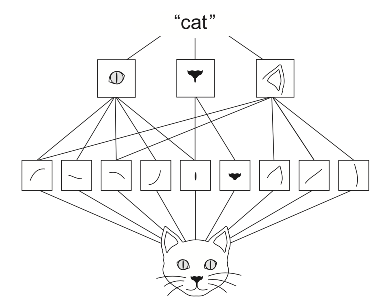
Spatial hierarchies

• Deep convnets can learn spatial hierarchies of patterns
  • First layer can learn very local patterns (e.g. edges)
  • Second layer can learn specific combinations of patterns
  • Every layer can learn increasingly complex abstractions

Visualizing the learned filters

• Visualize filters by finding the input image that they are maximally responsive to
• Gradient ascent in input space: learn what input maximizes the activations for that filter
  • Start from a random input image $X$, freeze the kernel
  • Loss = mean activation of output layer A, backpropagate to optimize $X$
  • $X_{(i+1)} = X_{(i)} + \frac{\partial L(x, X_{(i)})}{\partial X} * \eta$

Visualization: initialization (top) and after 100 optimization steps (bottom)

• Input image will show patterns that the filter responds to most

Gradient Ascent in input space in PyTorch

# Create a random input tensor and tell Adam to optimize the pixels
img = np.random.uniform(150, 180, (sz, sz, 3)) / 255
img_tensor.requires_grad_()
optimizer = optim.Adam([img_tensor], lr=lr, weight_decay=1e-6)

for _ in range(steps): 
    # Add our hook on the layer of interest to get the activations
    hook = layer.register_forward_hook(hook_fn) 
    
    # Run the input through the model
    model(img_tensor) 

    # Loss = Avg Activation of specific filter
    loss = -activations[0, filter_idx].mean()
    
    # Update inputs to maximize activation
    loss.backward() 
    optimizer.step()

• First layers respond mostly to colors, horizontal/diagonal edges
• Deeper layer respond to circular, triangular, stripy,... patterns

• We need to go deeper and train for much longer.
• Let's do this again for the VGG16 network pretrained on ImageNet

from torchvision.models import vgg16, VGG16_Weights
model = vgg16(weights=VGG16_Weights.IMAGENET1K_V1)

• First layers: very clear color and edge detectors
• 3rd layer responds to arcs, circles, sharp corners

• Deeper: more intricate patterns in different colors emerge
• Swirls, arches, boxes, circles,...

• Deeper: Filters specialize in all kinds of natural shapes
• More complex patterns (waves, landscapes, eyes) seem to appear

• Deepest layers have 512 filters each, each responding to very different patterns
• This 512-dimensional embedding separates distinct classes of images in 'feature space'

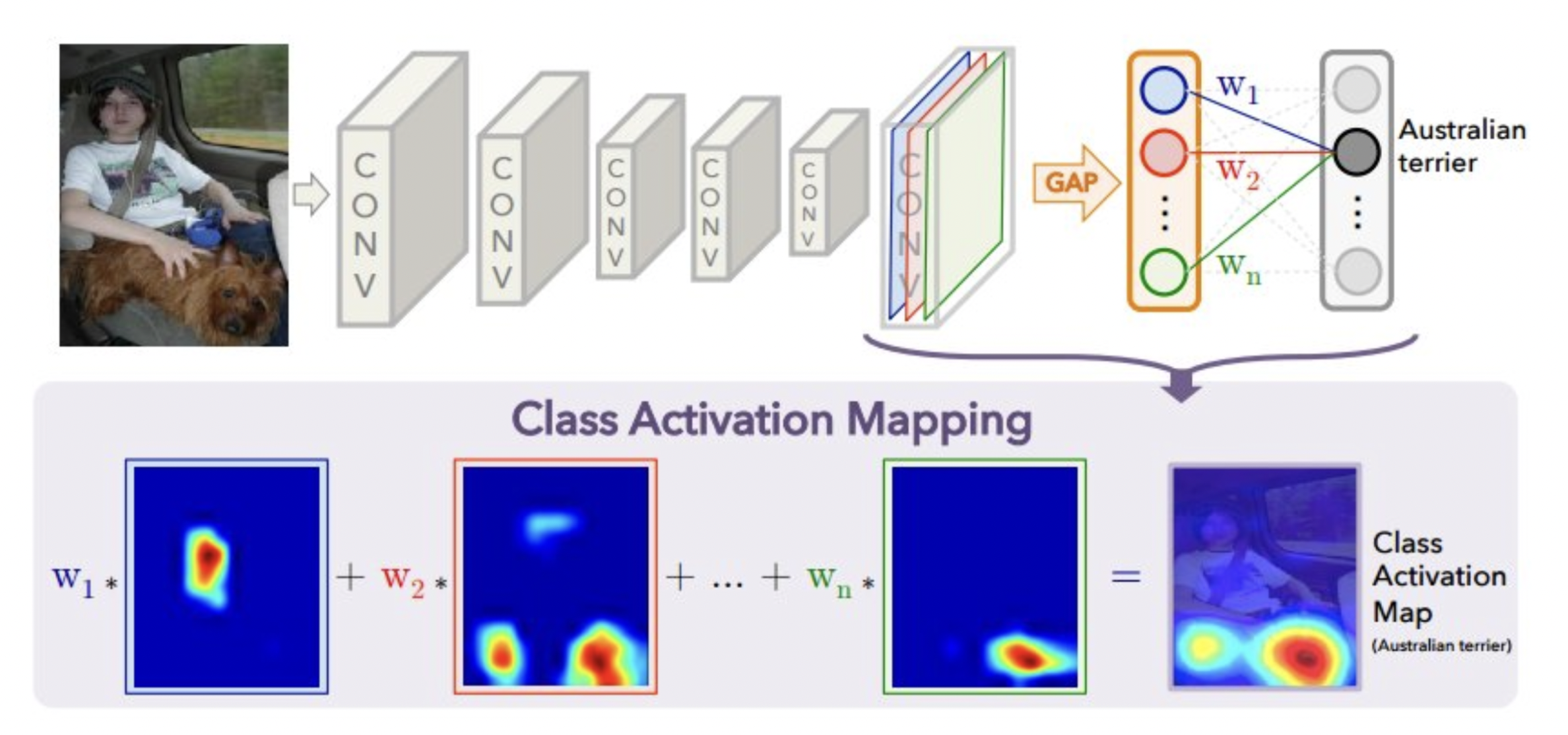
Visualizing class activation

• We can also visualize which pixels of the input had the greatest influence on the final classification. Helps to interpret what the model is paying attention to.
• Class activation maps : produces a heatmap over the input image
  • Choose a convolution layer, do Global Average Pooling (GAP) to get one output per channel
  • Get the weights between those outputs and the class of interest
  • Compute the weighted sum of all filter activations: combines what each filter is responding to and how much this affects the class prediction

Implementing gradCAM

    # Hooks to capture activations and gradients
    def forward_hook(module, input, output):
        activations = output
    def backward_hook(module, grad_input, grad_output):
        gradients = grad_output[0]
    target_layer.register_forward_hook(forward_hook)
    target_layer.register_full_backward_hook(backward_hook)

    # Forward pass + get predicted class
    pred_class = model(img_tensor).argmax(dim=1).item()

    # For that class, do a backward pass to get gradients
    model.zero_grad()
    output[:, pred_class].backward()

    # Compute Grad-CAM heatmap
    weights = torch.mean(gradients, dim=[2, 3], keepdim=True)  # GAP layer
    heatmap = torch.sum(weights * activations, dim=1).squeeze()

ResNet50 model, image of class Elephant, top-8 channels (highest weighst)

Transfer learning

• We can re-use pretrained networks instead of training from scratch
• Learned features can be a useful generic representation of the visual world
• General approach:
  • Remove the original classifier head and add a new one
  • Freeze the pretrained weights (backbone), then train as usual
  • Optionally unfreeze (and re-learn) part of the network

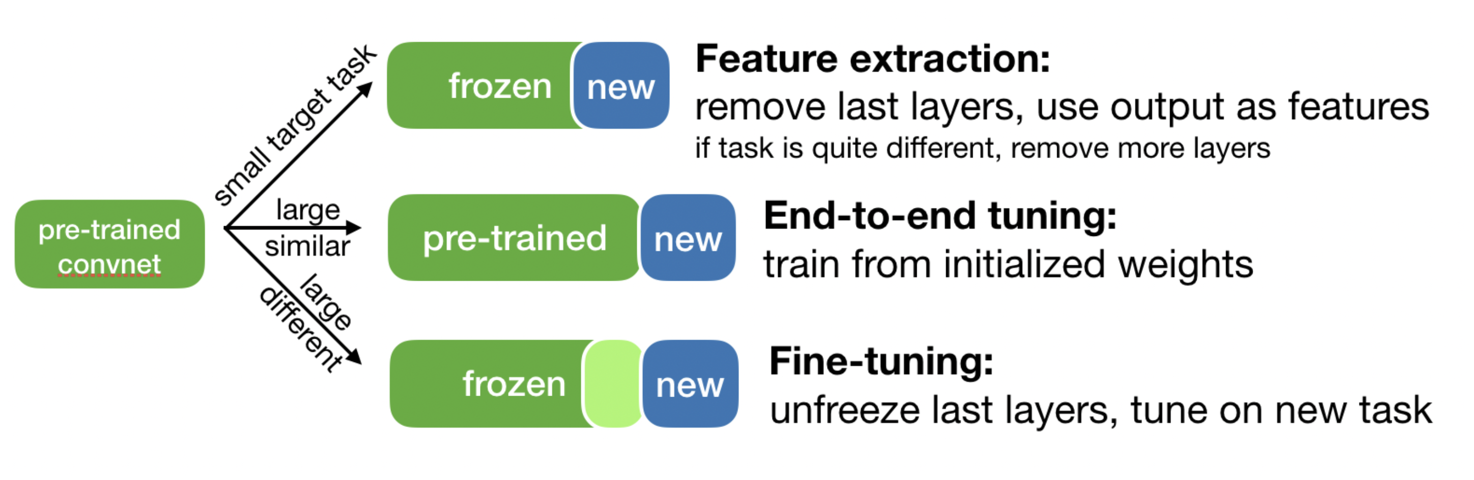
Using pre-trained networks: 3 ways

• Fast feature extraction (for similar task, little data)
  • Run data through convolutional base to build new features
  • Use embeddings as input to a dense layer (or another algorithm)
• End-to-end finetuning (for similar task, lots of data + data augmentation)
  • Extend the convolutional base model with a new dense layer
  • Train it end to end on the new data
• Partial fine-tuning (for somewhat different task)
  • Unfreeze a few of the top convolutional layers, and retrain
  • Update only the deeper (more task-specific layers)

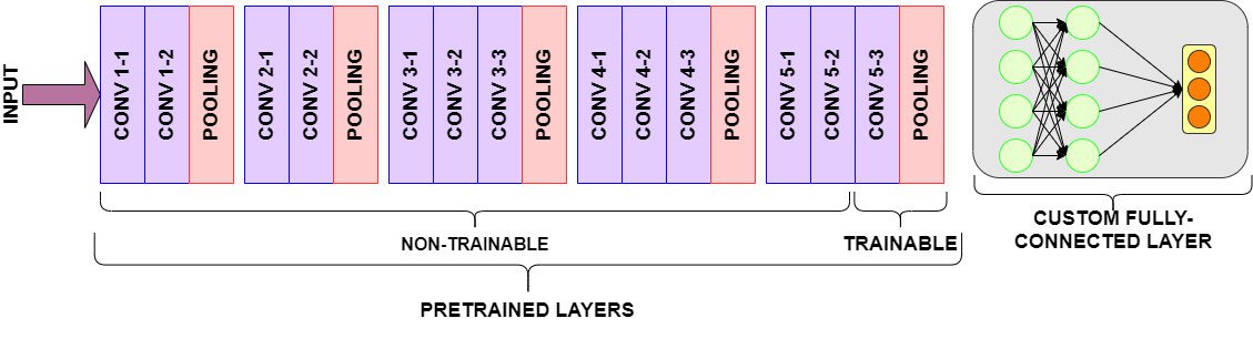
Fast feature extraction

• Pretrained ResNet18 architecture, remove fully-connected layers
• Add new classification head, freeze all pretrained weights

def __init__(self):
    resnet = resnet18(weights=ResNet18_Weights.IMAGENET1K_V1)
    self.feature_dim = resnet.fc.in_features
    self.resnet.fc = nn.Identity()                   # Remove old head
    self.classifier = nn.Linear(self.feature_dim, 1) # New head
    for param in self.backbone.parameters():  # Freeze backbone 
        param.requires_grad = False

# Train
def forward(self, x):
    features = self.resnet(x)
    logits = self.classifier(features)
    return logits.squeeze(1)

Fast feature extraction for cats and dogs

• Training from scratch (see earlier): 85% accuracy after 30 epochs
  • With transfer learning: 94% in a few epochs
• However, not much capacity for learning more (weights are frozen)
  • We could add more dense layers, but are stuck with the conv layers
• 512 trainable parameters

Partial finetuning

• Freeze backbone as before
• Unfreeze the last convolutional block

# Freeze conv layers 
for param in self.backbone.parameters():
    param.requires_grad = False
    
# Unfreeze last block 
for param in self.resnet.layer4.parameters():
    param.requires_grad = True

Partial finetuning for cats and dogs

• Performance increases to 96-97% accuracy in few epochs
• No further increase, and much overfitting (even with data augmentation)
  • More regularization needed to keep learning
• 8.4 million trainable parameters

End-to-end finetuning

• Freeze backbone as before. Unfreeze the last convolutional block
• Use a gentler initial learning rate for the backbone (to avoid destruction)

# Make conv layers trainable
for param in self.resnet.parameters():
    param.requires_grad = True

# Use a gentle learning rate for the backbone
def configure_optimizers(self):
    return torch.optim.Adam([
        {"params": self.resnet.parameters(), "lr": self.hparams.learning_rate * 0.1},
        {"params": self.classifier.parameters(), "lr": self.hparams.learning_rate}])

End-to-end finetuning for cats and dogs

• Very similar behavior, maybe slightly better, but also overfitting.
• Our dataset is likely too small to learn a better embedding
• 11.2 million trainable parameters

Take-aways

• 2D Convnets are ideal for addressing image-related problems.
  • 1D convnets are sometimes used for text, signals,...
• Compositionality: learn a hierarchy of simple to complex patterns
• Translation invariance: deeper networks are more robust to data variance
• Data augmentation helps fight overfitting (for small datasets)
• Representations are easy to inspect: visualize activations, filters, GradCAM
• Transfer learning: pre-trained embeddings can often be effectively reused to learn deep models for small datasets