Lecture 7. Bayesian Learning¶

Learning in an uncertain world

Joaquin Vanschoren

XKCD, Randall Monroe

Bayes' rule¶

Rule for updating the probability of a hypothesis $c$ given data $x$

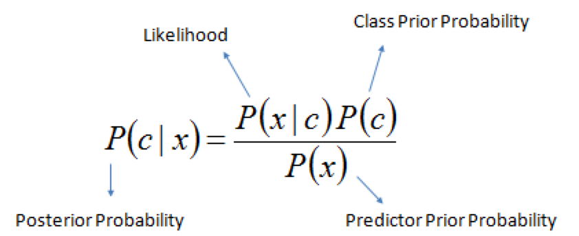
$P(c|x)$ is the posterior probability of class $c$ given data $x$.
$P(c)$ is the prior probability of class $c$: what you believed before you saw the data $x$
$P(x|c)$ is the likelihood of data point $x$ given that the class is $c$ (computed from your dataset)
$P(x)$ is the prior probability of the data (marginal likelihood): the likelihood of the data $x$ under any circumstance (no matter what the class is)

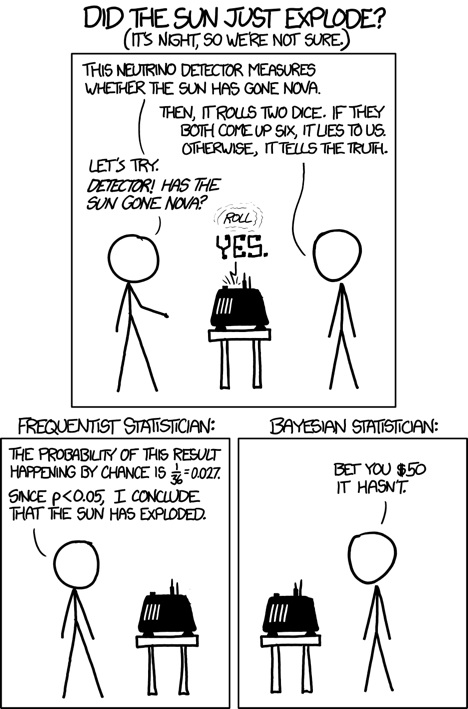
Example: exploding sun¶

Let's compute the probability that the sun has exploded
Prior $P(exploded)$: the sun has an estimated lifespan of 10 billion years, $P(exploded) = \frac{1}{4.38 x 10^{13}}$
Likelihood that detector lies: $P(lie)= \frac{1}{36}$

$$ \begin{aligned} P(exploded|yes) &= \frac{P(yes|exploded)P(exploded)}{P(yes)} \\ &= \frac{(1-P(lie)) P(exploded)}{P(exploded)(1-P(lie))+P(lie)(1-P(exploded))} \\ &= \frac{1}{1.25226 x 10^{12}} \end{aligned}$$

The one positive observation of the detector increases the probability

Example: COVID test¶

What is the probability of having COVID-19 if a 96% accurate test returns positive? Assume a false positive rate of 4%
Prior $P(C): 0.015$ (117M cases, 7.9B people)
$P(TP)=P(pos|C)=0.96$, and $P(FP)=(pos|notC)=0.04$
If test is positive, prior becomes $P(C)=0.268$. 2nd positive test: $P(C|pos)=0.9$

$$ \begin{aligned} P(C|pos) &= \frac{P(pos|C)P(C)}{P(pos)} \\ &= \frac{P(pos|C) P(C)}{P(pos|C)P(C)+P(pos|notC)(1-P(C))} \\ &= \frac{0.96*0.015}{0.96*0.015+0.04*0.985} \\ &= 0.268 \end{aligned}$$

Bayesian models¶

Learn the joint distribution $P(x,y)=P(x|y)P(y)$.
- Assumes that the data is Gaussian distributed (!)
- With every input $x$ you get $P(y|x)$, hence a mean and standard deviation for $y$ (blue)
- For every desired output $y$ you get $P(x|y)$, hence you can sample new points $x$ (red)
Easily updatable with new data using Bayes' rule ('turning the crank')
- Previous posterior $P(y|x)$ becomes new prior $P(y)$

interactive(children=(FloatSlider(value=0.0, description='x', max=3.0, min=-3.0, step=0.5), FloatSlider(value=…

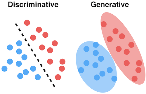
Generative models¶

The joint distribution represents the training data for a particular output (e.g. a class)
You can sample a new point $\textbf{x}$ with high predicted likelihood $P(x,c)$: that new point will be very similar to the training points
Generate new (likely) points according to the same distribution: generative model
- Generate examples that are fake but corresponding to a desired output
- Generative neural networks (e.g. GANs) can do this very accurately for text, images, ...

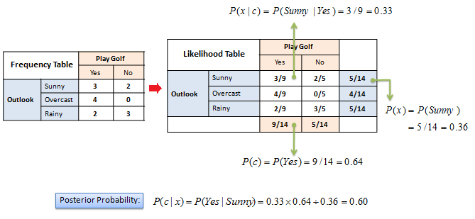
Naive Bayes¶

Predict the probability that a point belongs to a certain class, using Bayes' Theorem

$$P(c|\textbf{x}) = \frac{P(\textbf{x}|c)P(c)}{P(\textbf{x})}$$

Problem: since $\textbf{x}$ is a vector, computing $P(\textbf{x}|c)$ can be very complex
Naively assume that all features are conditionally independent from each other, in which case:
$P(\mathbf{x}|c) = P(x_1|c) \times P(x_2|c) \times ... \times P(x_n|c)$
Very fast: only needs to extract statistics from each feature.

On categorical data¶

What's the probability that your friend will play golf if the weather is sunny?

On numeric data¶

We need to fit a distribution (e.g. Gaussian) over the data points
GaussianNB: Computes mean $\mu_c$ and standard deviation $\sigma_c$ of the feature values per class: $p(x=v \mid c)=\frac{1}{\sqrt{2\pi\sigma^2_c}}\,e^{ -\frac{(v-\mu_c)^2}{2\sigma^2_c} }$
We can now make predictions using Bayes' theorem: $p(c \mid \mathbf{x}) = \frac{p(\mathbf{x} \mid c) \ p(c)}{p(\mathbf{x})}$

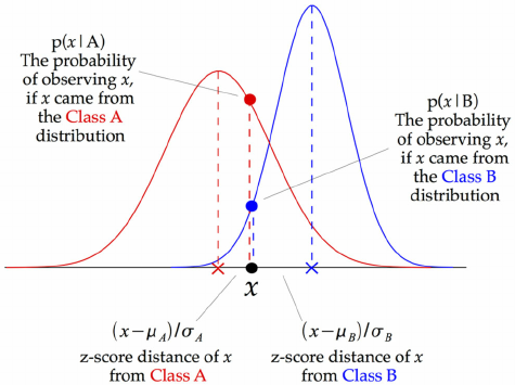
What do the predictions of Gaussian Naive Bayes look like?

Other Naive Bayes classifiers:

BernoulliNB
- Assumes binary data
- Feature statistics: Number of non-zero entries per class
MultinomialNB
- Assumes count data
- Feature statistics: Average value per class
- Mostly used for text classification (bag-of-words data)

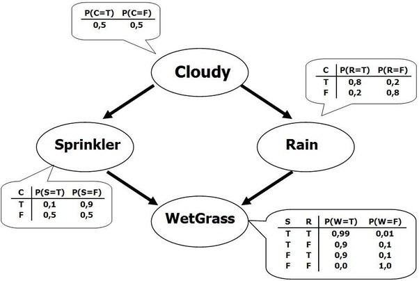
Bayesian Networks¶

What if we know that some variables are not independent?
A Bayesian Network is a directed acyclic graph representing variables as nodes and conditional dependencies as edges.
If an edge $(A, B)$ connects random variables A and B, then $P(B|A)$ is a factor in the joint probability distribution. We must know $P(B|A)$ for all values of $B$ and $A$
The graph structure can be designed manually or learned (hard!)

Gaussian processes¶

Model the data as a Gaussian distribution, conditioned on the training points

interactive(children=(IntSlider(value=10, description='nr_points', max=20), Output()), _dom_classes=('widget-i…

Probabilistic interpretation of regression¶

Linear regression (recap):

$$y = f(\mathbf{x}_i) = \mathbf{x}_i\mathbf{w} + b $$

For one input feature: $$y = w_1 \cdot x_1 + b \cdot 1$$

We can solve this via linear algebra (closed form solution): $w^{*} = (X^{T}X)^{-1} X^T Y$

w = np.linalg.solve(np.dot(X.T, X), np.dot(X.T, y))

$\mathbf{X}$ is our data matrix with a $x_0=1$ column to represent the bias $b$:

$$\mathbf{X} = \begin{bmatrix} \mathbf{x}_1^\top \\\ \mathbf{x}_2^\top \\\ \vdots \\\ \mathbf{x}_N^\top \end{bmatrix} = \begin{bmatrix} 1 & x_1 \\\ 1 & x_2 \\\ \vdots & \vdots \\\ 1 & x_N \end{bmatrix}$$

Example: Olympic marathon data¶

We learned: $ y= w_1 x + w_0 = -0.013 x + 28.895$

Polynomial regression (recap)¶

We can fit a 2nd degree polynomial by using a basis expansion (adding more basis functions):

$$\mathbf{\Phi} = \left[ \mathbf{1} \quad \mathbf{x} \quad \mathbf{x}^2\right]$$

Kernelized regression (recap)¶

We can also kernelize the model and learn a dual coefficient per data point

interactive(children=(IntSlider(value=4, description='poly_degree', max=8, min=1), IntSlider(value=-6, descrip…

Probabilistic interpretation¶

These models do not give us any indication of the (un)certainty of the predictions
Assume that the data is inherently uncertain. This can be modeled explictly by introducing a slack variable, $\epsilon_i$, known as noise.

$$y_i = w_1 x_i + w_0 + \epsilon_i.$$

Assume that the noise is distributed according to a Gaussian distribution with zero mean and variance $\sigma^2$.

$$\epsilon_i \sim \mathcal{N}(0, \sigma^2)$$

That means that $y(x)$ is now a Gaussian distribution with mean $\mathbf{wx}$ and variance $\sigma^2$

$$y = \mathcal{N}(\mathbf{wx}, \sigma^2)$$

We have an uncertainty predictions, but it is the same for all predictions

You would expect to be more certain nearby your training points

interactive(children=(FloatSlider(value=0.005, description='sigma', max=0.01, min=0.001, step=0.001), Output()…

How to learn probabilities?¶

Maximum Likelihood Estimation (MLE): Maximize $P(\textbf{X}|\textbf{w})$
- Corresponds to optimizing $\mathbf{w}$, using (log) likelihood as the loss function
- Every prediction has a mean defined by $\textbf{w}$ and Gaussian noise $$P(\textbf{X}|\textbf{w}) = \prod_{i=0}^{n} P(\mathbf{y}_i|\mathbf{x}_i;\mathbf{w}) = \prod_{i=0}^{n} \mathcal{N}(\mathbf{wx,\sigma^2 I})$$

Maximum A Posteriori estimation (MAP): Maximize the posterior $P(\textbf{w}|\textbf{X})$
- This can be done using Bayes' rule after we choose a (Gaussian) prior $P(\textbf{w})$: $$P(\textbf{w}|\textbf{X}) = \frac{P(\textbf{X}|\textbf{w})P(\textbf{w})}{P(\textbf{X})}$$
Bayesian approach: model the prediction $P(y|x_{test},X)$ directly
- Marginalize $w$ out: consider all possible models (some are more likely)
- If prior $P(\textbf{w})$ is Gaussian, then $P(y|x_{test},\textbf{X})$ is also Gaussian!
  - A multivariate Gaussian with mean $\mu$ and covariance matrix $\Sigma$ $$P(y|x_{test},\textbf{X}) = \int_w P(y|x_{test},\textbf{w}) P(\textbf{w}|\textbf{X}) dw = \mathcal{N}(\mathbf{\mu,\Sigma})$$

Gaussian prior $P(w)$¶

In the Bayesian approach, we assume a prior (Gaussian) distribution for the parameters, $\mathbf{w} \sim \mathcal{N}(\mathbf{0}, \alpha \mathbf{I})$:

With zero mean ($\mu$=0) and covariance matrix $\alpha \mathbf{I}$. For 2D: $ \alpha \mathbf{I} = \begin{bmatrix} \alpha & 0 \\ 0 & \alpha \end{bmatrix}$

I.e, $w_i$ is drawn from a Gaussian density with variance $\alpha$ $$w_i \sim \mathcal{N}(0,\alpha)$$

interactive(children=(FloatSlider(value=0.5, description='alpha', max=1.0, min=0.1), Checkbox(value=False, des…

Sampling from the prior (weight space)¶

We can sample from the prior distribution to see what form we are imposing on the functions a priori (before seeing any data).

Draw $w$ (left) independently from a Gaussian density $\mathbf{w} \sim \mathcal{N}(\mathbf{0}, \alpha\mathbf{I})$
- Use any normally distributed sampling technique, e.g. Box-Mueller transform
Every sample yields a polynomial function $f(\mathbf{x})$ (right): $f(\mathbf{x}) = \mathbf{w} \boldsymbol{\phi}(\mathbf{x}).$
- For example, with $\boldsymbol{\phi}(\mathbf{x})$ being a polynomial:

interactive(children=(FloatSlider(value=2.1, description='alpha', max=5.0, min=0.1, step=0.5), IntSlider(value…

Learning Gaussian distributions¶

We assume that our data is Gaussian distributed: $P(y|x_{test},\textbf{X}) = \mathcal{N}(\mathbf{\mu,\Sigma})$
Example with learned mean $[m,m]$ and covariance $\begin{bmatrix} \alpha & \beta \\ \beta & \alpha \end{bmatrix}$
- The blue curve is the predicted $P(y|x_{test},\textbf{X})$

interactive(children=(FloatSlider(value=0.0, description='x_test', max=3.0, min=-3.0, step=0.5), FloatSlider(v…

Understanding covariances¶

If two variables $x_i$ covariate strongly, knowing about $x_1$ tells us a lot about $x_2$
If covariance is 0, knowing $x_1$ tells us nothing about $x_2$ (the conditional and marginal distributions are the same)
For covariance matrix $\begin{bmatrix} 1 & \beta \\ \beta & 1 \end{bmatrix}$:

interactive(children=(FloatSlider(value=0.0, description='x1', max=3.0, min=-3.0, step=0.5), FloatSlider(value…

Sampling from higher-dimensional distributions¶

Instead of sampling $\mathbf{w}$ and then multiplying by $\boldsymbol{\Phi}$, we can also generate examples of $f(x)$ directly.
$\mathbf{f}$ with $n$ values can be sampled from an $n$-dimensional Gaussian distribution with zero mean and covariance matrix $\mathbf{K} = \alpha \boldsymbol{\Phi}\boldsymbol{\Phi}^\top$:
- $\mathbf{f}$ is a stochastic process: series of normally distributed variables (interpolated in the plot)

$$\mathbf{f} \sim \mathcal{N}(\mathbf{0},\mathbf{K})$$

interactive(children=(FloatSlider(value=1.0, description='alpha', max=2.0, min=0.1), IntSlider(value=51, descr…

Repeat for 40 dimensions, with $\boldsymbol{\Phi}$ the polynomial transform:

More examples of covariances

Noisy functions¶

We normally add Gaussian noise to obtain our observations: $$ \mathbf{y} = \mathbf{f} + \boldsymbol{\epsilon} $$

interactive(children=(FloatSlider(value=0.05, description='sigma', max=0.1, min=0.01, step=0.01), Output()), _…

Gaussian Process¶

Usually, we want our functions to be smooth: if two points are similar/nearby, the predictions should be similar.
- Hence, we need a similarity measure (a kernel)
In a Gaussian process we can do this by specifying the covariance function directly (not as $\mathbf{K} = \alpha \boldsymbol{\Phi}\boldsymbol{\Phi}^\top$)
- The covariance matrix is simply the kernel matrix: $\mathbf{f} \sim \mathcal{N}(\mathbf{0},\mathbf{K})$
The RBF (Gaussian) covariance function (or kernel) is specified by

$$ k(\mathbf{x}, \mathbf{x}^\prime) = \alpha \exp\left( -\frac{\left\Vert \mathbf{x}-\mathbf{x}^\prime\right\Vert^2}{2\ell^2}\right). $$

where $\left\Vert\mathbf{x} - \mathbf{x}^\prime\right\Vert^2$ is the squared distance between the two input vectors

$$ \left\Vert\mathbf{x} - \mathbf{x}^\prime\right\Vert^2 = (\mathbf{x} - \mathbf{x}^\prime)^\top (\mathbf{x} - \mathbf{x}^\prime) $$

and the length parameter $l$ controls the smoothness of the function and $\alpha$ the vertical variation.

Now the influence of a point decreases smoothly but exponentially

These are our priors $P(y) = \mathcal{N}(\mathbf{0,\mathbf{K}})$, with mean 0
We now want to condition it on our training data: $P(y|x_{test},\textbf{X}) = \mathcal{N}(\mathbf{\mu,\Sigma})$

interactive(children=(FloatSlider(value=1.0, description='alpha', max=2.0, min=0.1), IntSlider(value=10, descr…

Computing the posterior $P(\mathbf{y}|\mathbf{X})$¶

Assuming that $P(X)$ is a Gaussian density with a covariance given by kernel matrix $\mathbf{K}$, the model likelihood becomes: $$ P(\mathbf{y}|\mathbf{X}) = \frac{P(y) \ P(\mathbf{X} \mid y)}{P(\mathbf{X})} = \frac{1}{(2\pi)^{\frac{n}{2}}|\mathbf{K}|^{\frac{1}{2}}} \exp\left(-\frac{1}{2}\mathbf{y}^\top \left(\mathbf{K}+\sigma^2 \mathbf{I}\right)^{-1}\mathbf{y}\right) $$
Hence, the negative log likelihood (the objective function) is given by: $$ E(\boldsymbol{\theta}) = \frac{1}{2} \log |\mathbf{K}| + \frac{1}{2} \mathbf{y}^\top \left(\mathbf{K} + \sigma^2\mathbf{I}\right)^{-1}\mathbf{y} $$
The model parameters (e.g. noise variance $\sigma^2$) and the kernel parameters (e.g. lengthscale, variance) can be embedded in the covariance function and learned from data.
Good news: This loss function can be optimized using linear algebra (Cholesky Decomposition)
Bad news: This is cubic in the number of data points AND the number of features: $\mathcal{O}(n^3 d^3)$

Making predictions¶

The model makes predictions for $\mathbf{f}$ that are unaffected by future values of $\mathbf{f}^*$.
If we think of $\mathbf{f}^*$ as test points, we can still write down a joint probability density over the training observations, $\mathbf{f}$ and the test observations, $\mathbf{f}^*$.

This joint probability density will be Gaussian, with a covariance matrix given by our kernel function, $k(\mathbf{x}_i, \mathbf{x}_j)$. $$ \begin{bmatrix}\mathbf{f} \\ \mathbf{f}^*\end{bmatrix} \sim \mathcal{N}\left(\mathbf{0}, \begin{bmatrix} \mathbf{K} & \mathbf{K}_\ast \\ \mathbf{K}_\ast^\top & \mathbf{K}_{\ast,\ast}\end{bmatrix}\right) $$

where $\mathbf{K}$ is the kernel matrix computed between all the training points,
$\mathbf{K}_\ast$ is the kernel matrix computed between the training points and the test points,
$\mathbf{K}_{\ast,\ast}$ is the kernel matrix computed between all the tests points and themselves.

Conditional Density $P(\mathbf{y}|x_{test} , \mathbf{X})$¶

Finally, we need to define conditional distributions to answer particular questions of interest

We will need the conditional density for making predictions. $$ \mathbf{f}^* | \mathbf{y} \sim \mathcal{N}(\boldsymbol{\mu}_f,\mathbf{C}_f) $$ with a mean given by $ \boldsymbol{\mu}_f = \mathbf{K}_*^\top \left[\mathbf{K} + \sigma^2 \mathbf{I}\right]^{-1} \mathbf{y} $

and a covariance given by $ \mathbf{C}_f = \mathbf{K}_{*,*} - \mathbf{K}_*^\top \left[\mathbf{K} + \sigma^2 \mathbf{I}\right]^{-1} \mathbf{K}_\ast. $

interactive(children=(IntSlider(value=13, description='nr_points', max=27), Output()), _dom_classes=('widget-i…

Remember that our prediction is the sum of the mean and the variance: $P(\mathbf{y}|x_{test} , \mathbf{X}) = \mathcal{N}(\mathbf{\mu,\Sigma})$

The mean is the same as the one computed with kernel ridge (if given the same kernel and hyperparameters)
The Gaussian process learned the covariance and the hyperparameters

interactive(children=(IntSlider(value=13, description='nr_points', max=27), Checkbox(value=False, description=…

The values on the diagonal of the covariance matrix give us the variance, so we can simply plot the mean and 95% confidence interval

interactive(children=(IntSlider(value=13, description='nr_points', max=27), IntSlider(value=12, description='l…

Gaussian Processes in practice (with GPy)¶

GPyRegression
Generate a kernel first
- State the dimensionality of your input data
- Variance and lengthscale are optional, default = 1
```
kernel = GPy.kern.RBF(input_dim=1, variance=1., lengthscale=1.)
```
- Other kernels:
```
GPy.kern.BasisFuncKernel?
```
Build model:

m = GPy.models.GPRegression(X,Y,kernel)

Matern is a generalized RBF kernel that can scale between RBF and Exponential

Build the untrained GP. The shaded region corresponds to ~95% confidence intervals (i.e. +/- 2 standard deviation)

Train the model (optimize the parameters): maximize the likelihood of the data.
Best to optimize with a few restarts: the optimizer may converges to the high-noise solution. The optimizer is then restarted with a few random initialization of the parameter values.

You can also show results in 2D

We can plot 2D slices using the fixed_inputs argument to the plot function.
fixed_inputs is a list of tuples containing which of the inputs to fix, and to which value.

Gaussian Processes with scikit-learn¶

GaussianProcessRegressor
Hyperparameters:
- kernel: kernel specifying the covariance function of the GP
  - Default: "1.0 * RBF(1.0)"
  - Typically leave at default. Will be optimized during fitting
- alpha: regularization parameter
  - Tikhonov regularization of covariance between the training points.
  - Adds a (small) value to diagonal of the kernel matrix during fitting.
  - Larger values:
    - correspond to increased noise level in the observations
    - also reduce potential numerical issues during fitting
  - Default: 1e-10
- n_restarts_optimizer: number of restarts of the optimizer
  - Default: 0. Best to do at least a few iterations.
  - Optimizer finds kernel parameters maximizing log-marginal likelihood
Retrieve predictions and confidence interval after fitting:
```
y_pred, sigma = gp.predict(x, return_std=True)
```

Example

Example with noisy data

Gaussian processes: Conclusions¶

Advantages:

The prediction is probabilistic (Gaussian) so that one can compute empirical confidence intervals.
The prediction interpolates the observations (at least for regular kernels).
Versatile: different kernels can be specified.

Disadvantages:

They are typically not sparse, i.e., they use the whole sample/feature information to perform the prediction.
- Sparse GPs also exist: they remember only the most important points
They lose efficiency in high dimensional spaces – namely when the number of features exceeds a few dozens.

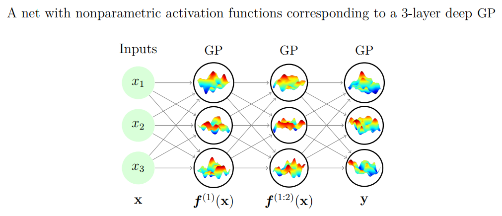
Gaussian processes and neural networks¶

You can prove that a Gaussian process is equivalent to a neural network with one layer and an infinite number of nodes
You can build deep Gaussian Processes by constructing layers of GPs

Bayesian optimization¶

The incremental updates you can do with Bayesian models allow a more effective way to optimize functions
- E.g. to optimize the hyperparameter settings of a machine learning algorithm/pipeline
After a number of random search iterations we know more about the performance of hyperparameter settings on the given dataset
We can use this data to train a model, and predict which other hyperparameter values might be useful
- More generally, this is called model-based optimization
- This model is called a surrogate model
This is often a probabilistic (e.g. Bayesian) model that predicts confidence intervals for all hyperparameter settings
We use the predictions of this model to choose the next point to evaluate
With every new evaluation, we update the surrogate model and repeat

Example (see figure):¶

Consider only 1 continuous hyperparameter (X-axis)
- You can also do this for many more hyperparameters
Y-axis shows cross-validation performance
Evaluate a number of random hyperparameter settings (black dots)
- Sometimes an initialization design is used
Train a model, and predict the expected performance of other (unseen) hyperparameter values
- Mean value (black line) and distribution (blue band)
An acquisition function (green line) trades off maximal expected performace and maximal uncertainty
- Exploitation vs exploration
Optimal value of the asquisition function is the next hyperparameter setting to be evaluated
Repeat a fixed number of times, or until time budget runs out

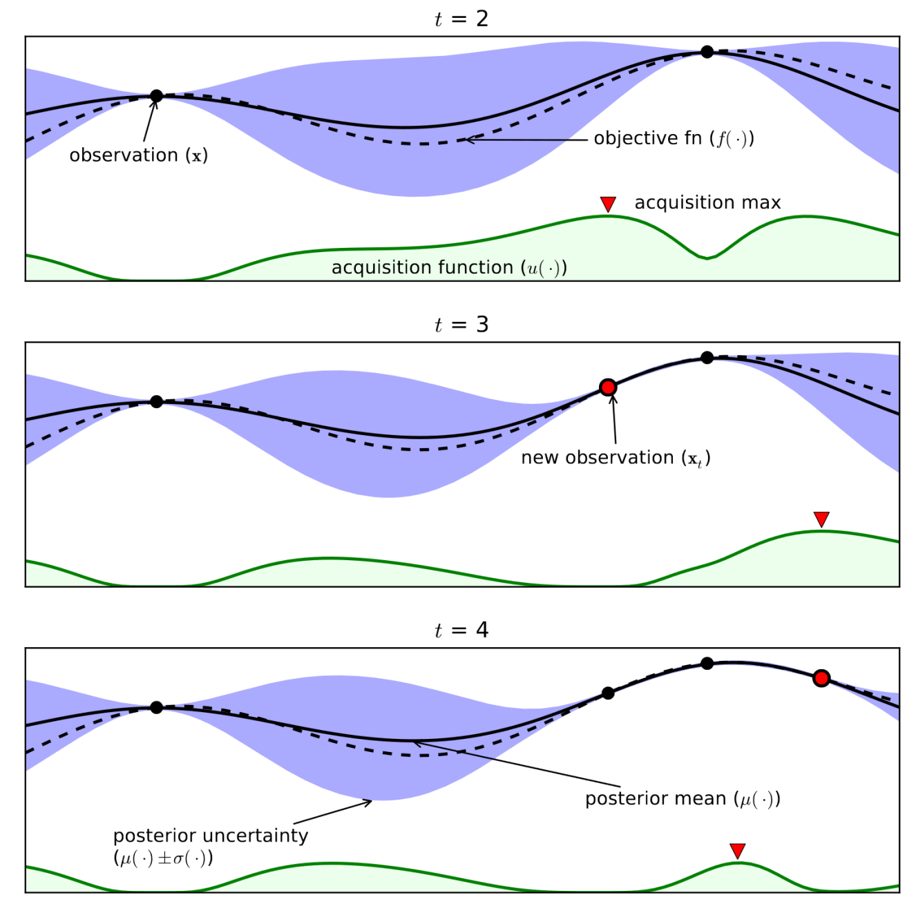
Shahriari et al. Taking the Human Out of the Loop: A Review of Bayesian Optimization

In 2 dimensions:

Surrogate models¶

Surrogate model can be anything as long as it can do regression and is probabilistic
Gaussian Processes are commonly used
- Smooth, good extrapolation, but don't scale well to many hyperparameters (cubic)
- Sparse GPs: select ‘inducing points’ that minimize info loss, more scalable
- Multi-task GPs: transfer surrogate models from other tasks
Random Forests
- A lot more scalable, but don't extrapolate well
- Often an interpolation between predictions is used instead of the raw (step-wise) predictions
Bayesian Neural Networks:
- Expensive, sensitive to hyperparameters

Acquisition Functions¶

When we have trained the surrogate model, we ask it to predict a number of samples
- Can be simply random sampling
- Better: Thompson sampling
  - fit a Gaussian distribution (a mixture of Gaussians) over the sampled points
  - sample new points close to the means of the fitted Gaussians
Typical acquisition function: Expected Improvement
- Models the predicted performance as a Gaussian distribution with the predicted mean and standard deviation
- Computes the expected performance improvement over the previous best configuration $\mathbf{X^+}$: $$EI(X) := \mathbb{E}\left[ \max\{0, f(\mathbf{X^+}) - f_{t+1}(\mathbf{X}) \} \right]$$
- Computing the expected performance requires an integration over the posterior distribution, but has a closed form solution.

Bayesian Optimization: conclusions¶

More efficient way to optimize hyperparameters
More similar to what humans would do
Harder to parallellize
Choice of surrogate model depends on your search space
- Very active research area
- For very high-dimensional search spaces, random forests are popular