Overview
- Neural architectures
- Training neural nets
- Forward pass: Tensor operations
- Backward pass: Backpropagation
- Neural network design:
- Activation functions
- Weight initialization
- Optimizers
- Neural networks in practice
- Model selection
- Early stopping
- Memorization capacity and information bottleneck
- L1/L2 regularization
- Dropout
- Batch normalization
Architecture
- Logistic regression, drawn in a different, neuro-inspired, way
- Linear model: inner product ($z$) of input vector $\mathbf{x}$ and weight vector $\mathbf{w}$, plus bias $w_0$
- Logistic (or sigmoid) function maps the output to a probability in [0,1]
- Uses log loss (cross-entropy) and gradient descent to learn the weights
$$\hat{y}(\mathbf{x}) = \text{sigmoid}(z) = \text{sigmoid}(w_0 + \mathbf{w}\mathbf{x}) = \text{sigmoid}(w_0 + w_1 * x_1 + w_2 * x_2 +... + w_p * x_p)$$

Basic Architecture
- Add one (or more) hidden layers $h$ with $k$ nodes (or units, cells, neurons)
- Every 'neuron' is a tiny function, the network is an arbitrarily complex function
- Weights $w_{i,j}$ between node $i$ and node $j$ form a weight matrix $\mathbf{W}^{(l)}$ per layer $l$
- Every neuron weights the inputs $\mathbf{x}$ and passes it through a non-linear activation function
- Activation functions ($f,g$) can be different per layer, output $\mathbf{a}$ is called activation $$\color{blue}{h(\mathbf{x})} = \color{blue}{\mathbf{a}} = f(\mathbf{z}) = f(\mathbf{W}^{(1)} \color{green}{\mathbf{x}}+\mathbf{w}^{(1)}_0) \quad \quad \color{red}{o(\mathbf{x})} = g(\mathbf{W}^{(2)} \color{blue}{\mathbf{a}}+\mathbf{w}^{(2)}_0)$$

More layers
- Add more layers, and more nodes per layer, to make the model more complex
- For simplicity, we don't draw the biases (but remember that they are there)
- In dense (fully-connected) layers, every previous layer node is connected to all nodes
- The output layer can also have multiple nodes (e.g. 1 per class in multi-class classification)

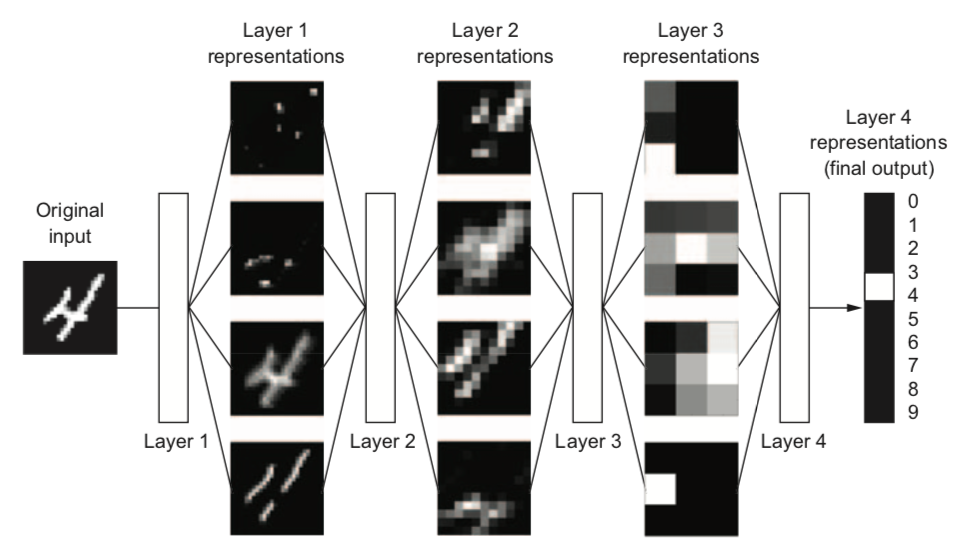
Why layers?
- Each layer acts as a filter and learns a new representation of the data
- Subsequent layers can learn iterative refinements
- Easier than learning a complex relationship in one go
- Example: for image input, each layer yields new (filtered) images
- Can learn multiple mappings at once: weight tensor $\mathit{W}$ yields activation tensor $\mathit{A}$
- From low-level patterns (edges, end-points, ...) to combinations thereof
- Each neuron 'lights up' if certain patterns occur in the input
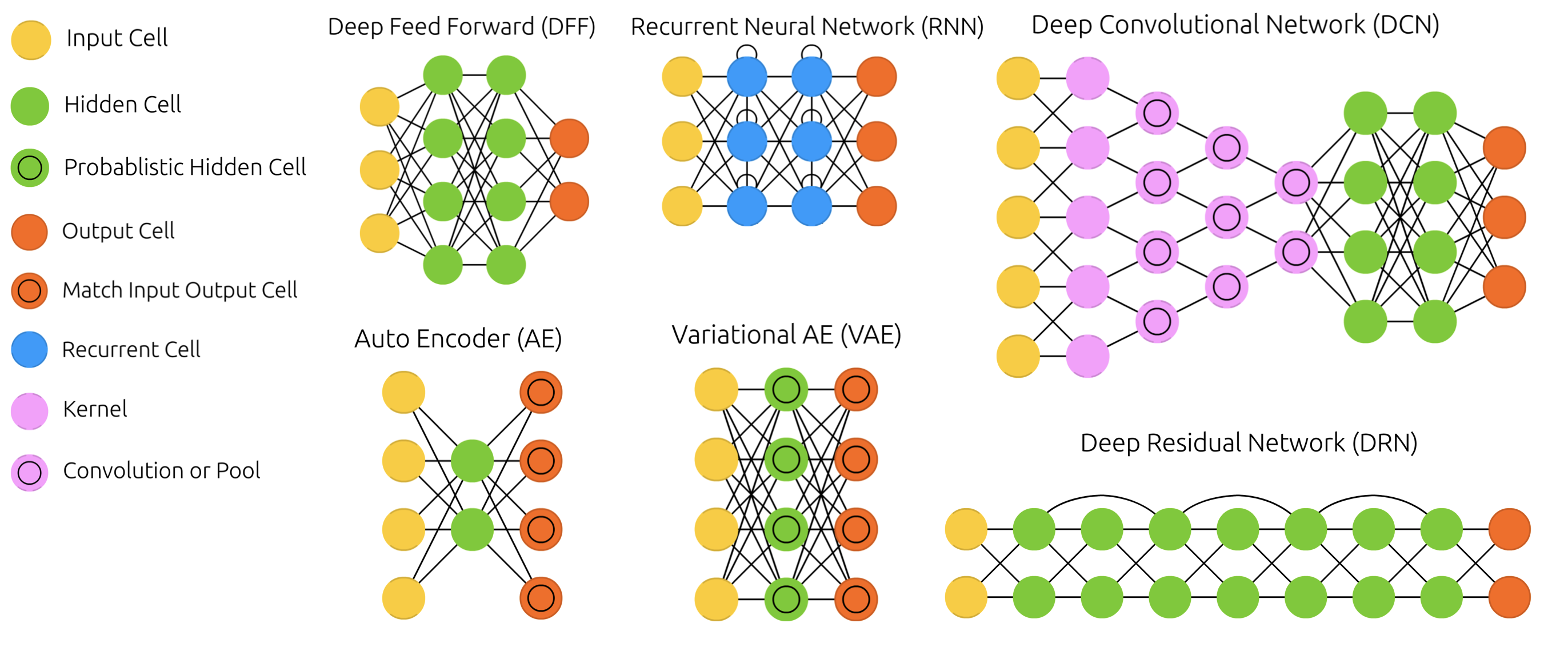
Other architectures
- There exist MANY types of networks for many different tasks
- Convolutional nets for image data, Recurrent nets for sequential data,...
- Also used to learn representations (embeddings), generate new images, text,...
Training Neural Nets
- Design the architecture, choose activation functions (e.g. sigmoids)
- Choose a way to initialize the weights (e.g. random initialization)
- Choose a loss function (e.g. log loss) to measure how well the model fits training data
- Choose an optimizer (typically an SGD variant) to update the weights
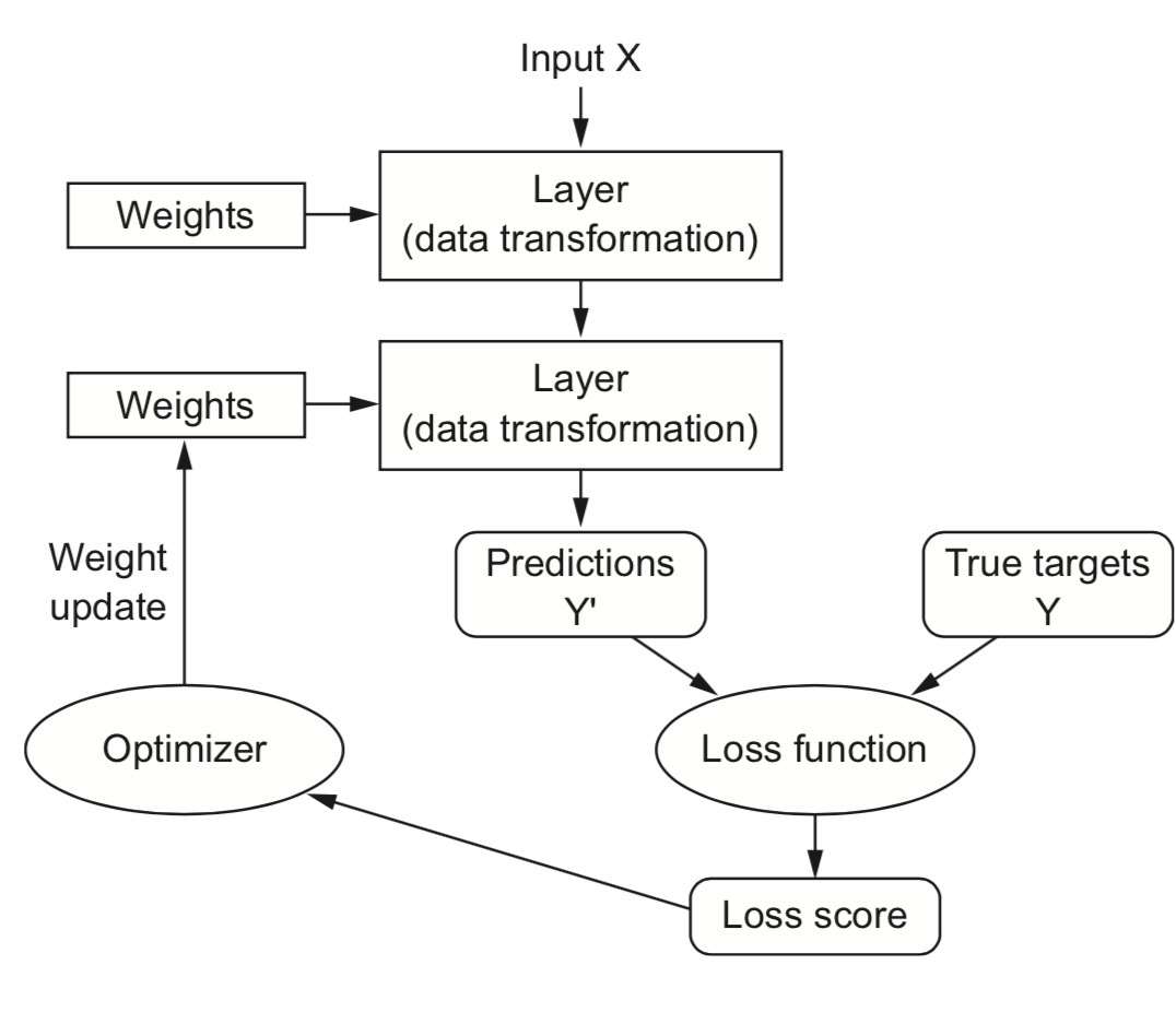
Mini-batch Stochastic Gradient Descent (recap)
- Draw a batch of batch_size training data $\mathbf{X}$ and $\mathbf{y}$
- Forward pass : pass $\mathbf{X}$ though the network to yield predictions $\mathbf{\hat{y}}$
- Compute the loss $\mathcal{L}$ (mismatch between $\mathbf{\hat{y}}$ and $\mathbf{y}$)
- Backward pass : Compute the gradient of the loss with regard to every weight
- Backpropagate the gradients through all the layers
- Update $W$: $W_{(i+1)} = W_{(i)} - \frac{\partial L(x, W_{(i)})}{\partial W} * \eta$
Repeat until n passes (epochs) are made through the entire training set

Forward pass
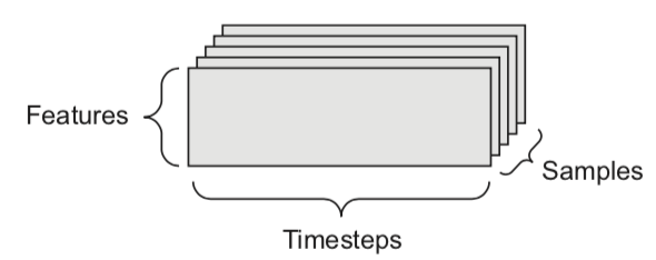
- We can naturally represent the data as tensors
- Numerical n-dimensional array (with n axes)
- 2D tensor: matrix (samples, features)
- 3D tensor: time series (samples, timesteps, features)
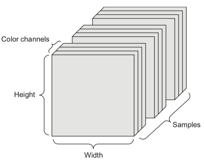
- 4D tensor: color images (samples, height, width, channels)
- 5D tensor: video (samples, frames, height, width, channels)
Tensor operations
- The operations that the network performs on the data can be reduced to a series of tensor operations
- These are also much easier to run on GPUs
- A dense layer with sigmoid activation, input tensor $\mathbf{X}$, weight tensor $\mathbf{W}$, bias $\mathbf{b}$:
y = sigmoid(np.dot(X, W) + b)
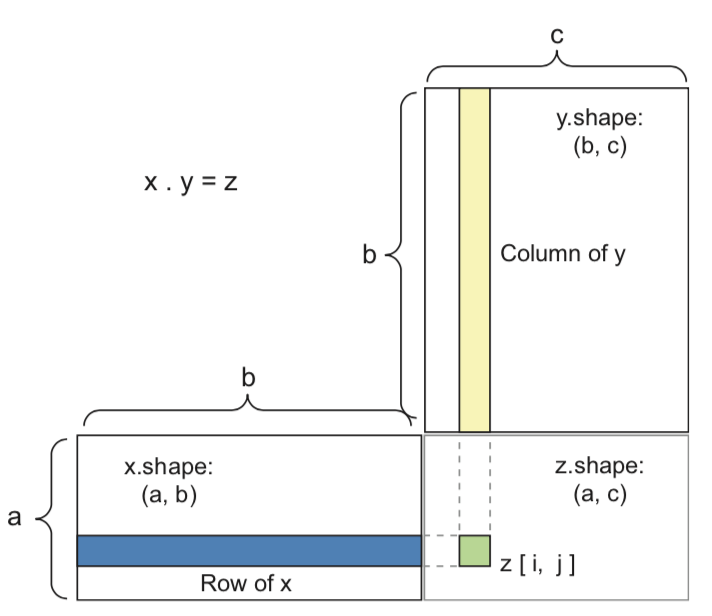
- Tensor dot product for 2D inputs ($a$ samples, $b$ features, $c$ hidden nodes)
Element-wise operations
- Activation functions and addition are element-wise operations:
def sigmoid(x):
  return 1/(1 + np.exp(-x))

def add(x, y):
  return x + y
- Note: if y has a lower dimension than x, it will be broadcasted: axes are added to match the dimensionality, and y is repeated along the new axes
>>> np.array([[1,2],[3,4]]) + np.array([10,20])
array([[11, 22],
       [13, 24]])
Backward pass (backpropagation)
- For last layer, compute gradient of the loss function $\mathcal{L}$ w.r.t all weights of layer $l$
$$\nabla \mathcal{L} = \frac{\partial \mathcal{L}}{\partial W^{(l)}} = \begin{bmatrix} \frac{\partial \mathcal{L}}{\partial w_{0,0}} & \ldots & \frac{\partial \mathcal{L}}{\partial w_{0,l}} \\ \vdots & \ddots & \vdots \\ \frac{\partial \mathcal{L}}{\partial w_{k,0}} & \ldots & \frac{\partial \mathcal{L}}{\partial w_{k,l}} \end{bmatrix}$$
- Sum up the gradients for all $\mathbf{x}_j$ in minibatch: $\sum_{j} \frac{\partial \mathcal{L}(\mathbf{x}_j,y_j)}{\partial W^{(l)}}$
- Update all weights in a layer at once (with learning rate $\eta$): $W_{(i+1)}^{(l)} = W_{(i)}^{(l)} - \eta \sum_{j} \frac{\partial \mathcal{L}(\mathbf{x}_j,y_j)}{\partial W_{(i)}^{(l)}}$
- Repeat for next layer, iterating backwards (most efficient, avoids redundant calculations)
Example
- Imagine feeding a single data point, output is $\hat{y} = g(z) = g(w_0 + w_1 * a_1 + w_2 * a_2 +... + w_p * a_p)$
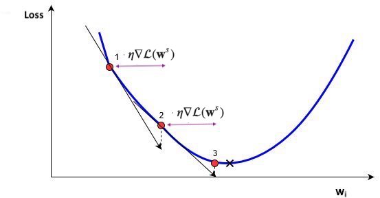
- Decrease loss by updating weights:
- Update the weights of last layer to maximize improvement: $w_{i,(new)} = w_{i} - \frac{\partial \mathcal{L}}{\partial w_i} * \eta$
- To compute gradient $\frac{\partial \mathcal{L}}{\partial w_i}$ we need the chain rule: $f(g(x)) = f'(g(x)) * g'(x)$ $$\frac{\partial \mathcal{L}}{\partial w_i} = \color{red}{\frac{\partial \mathcal{L}}{\partial g}} \color{blue}{\frac{\partial \mathcal{g}}{\partial z_0}} \color{green}{\frac{\partial \mathcal{z_0}}{\partial w_i}}$$
- E.g., with $\mathcal{L} = \frac{1}{2}(y-\hat{y})^2$ and sigmoid $\sigma$: $\frac{\partial \mathcal{L}}{\partial w_i} = \color{red}{(y - \hat{y})} * \color{blue}{\sigma'(z_0)} * \color{green}{a_i}$

Backpropagation (2)
- Another way to decrease the loss $\mathcal{L}$ is to update the activations $a_i$
- To update $a_i = f(z_i)$, we need to update the weights of the previous layer
- We want to nudge $a_i$ in the right direction by updating $w_{i,j}$: $$\frac{\partial \mathcal{L}}{\partial w_{i,j}} = \frac{\partial \mathcal{L}}{\partial a_i} \frac{\partial a_i}{\partial z_i} \frac{\partial \mathcal{z_i}}{\partial w_{i,j}} = \left( \frac{\partial \mathcal{L}}{\partial g} \frac{\partial \mathcal{g}}{\partial z_0} \frac{\partial \mathcal{z_0}}{\partial a_i} \right) \frac{\partial a_i}{\partial z_i} \frac{\partial \mathcal{z_i}}{\partial w_{i,j}}$$
- We know $\frac{\partial \mathcal{L}}{\partial g}$ and $\frac{\partial \mathcal{g}}{\partial z_0}$ from the previous step, $\frac{\partial \mathcal{z_0}}{\partial a_i} = w_i$, $\frac{\partial a_i}{\partial z_i} = f'$ and $\frac{\partial \mathcal{z_i}}{\partial w_{i,j}} = x_j$

Backpropagation (3)
- With multiple output nodes, $\mathcal{L}$ is the sum of all per-output (per-class) losses
- $\frac{\partial \mathcal{L}}{\partial a_i}$ is sum of the gradients for every output
- Per layer, sum up gradients for every point $\mathbf{x}$ in the batch: $\sum_{j} \frac{\partial \mathcal{L}(\mathbf{x}_j,y_j)}{\partial W}$
- Update all weights of every layer $l$
- $W_{(i+1)}^{(l)} = W_{(i)}^{(l)} - \eta \sum_{j} \frac{\partial \mathcal{L}(\mathbf{x}_j,y_j)}{\partial W_{(i)}^{(l)}}$
- Repeat with a new batch of data until loss converges
- Nice animation of the entire process

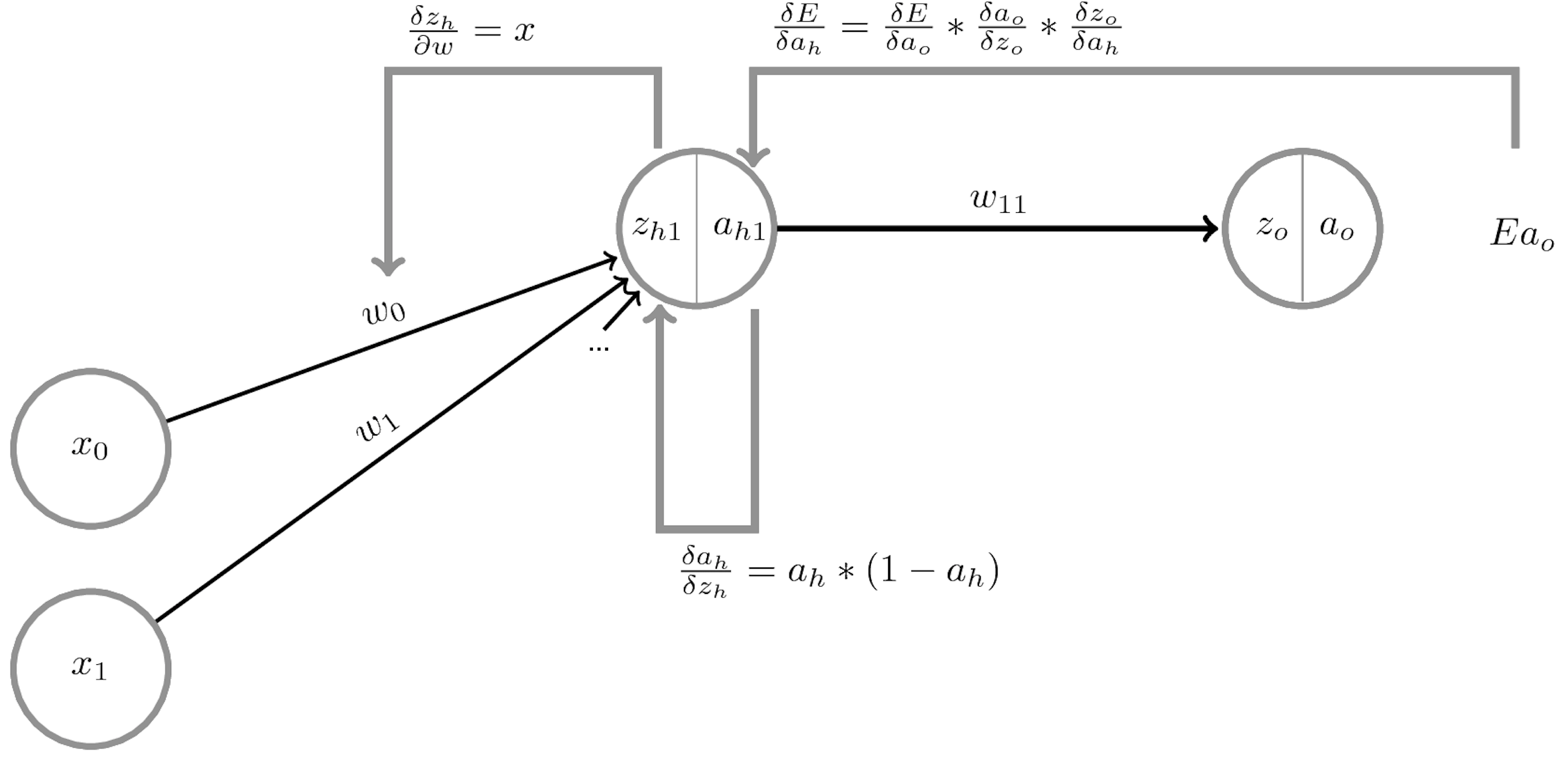
Summary
- The network output $a_o$ is defined by the weights $W^{(o)}$ and biases $\mathbf{b}^{(o)}$ of the output layer, and
- The activations of a hidden layer $h_1$ with activation function $a_{h_1}$, weights $W^{(1)}$ and biases $\mathbf{b^{(1)}}$:
$$\color{red}{a_o(\mathbf{x})} = \color{red}{a_o(\mathbf{z_0})} = \color{red}{a_o(W^{(o)}} \color{blue}{a_{h_1}(z_{h_1})} \color{red}{+ \mathbf{b}^{(o)})} = \color{red}{a_o(W^{(o)}} \color{blue}{a_{h_1}(W^{(1)} \color{green}{\mathbf{x}} + \mathbf{b}^{(1)})} \color{red}{+ \mathbf{b}^{(o)})} $$
- Minimize the loss by SGD. For layer $l$, compute $\frac{\partial \mathcal{L}(a_o(x))}{\partial W_l}$ and $\frac{\partial \mathcal{L}(a_o(x))}{\partial b_{l,i}}$ using the chain rule
- Decomposes into gradient of layer above, gradient of activation function, gradient of layer input:
$$\frac{\partial \mathcal{L}(a_o)}{\partial W^{(1)}} = \color{red}{\frac{\partial \mathcal{L}(a_o)}{\partial a_{h_1}}} \color{blue}{\frac{\partial a_{h_1}}{\partial z_{h_1}}} \color{green}{\frac{\partial z_{h_1}}{\partial W^{(1)}}} = \left( \color{red}{\frac{\partial \mathcal{L}(a_o)}{\partial a_o}} \color{blue}{\frac{\partial a_o}{\partial z_o}} \color{green}{\frac{\partial z_o}{\partial a_{h_1}}}\right) \color{blue}{\frac{\partial a_{h_1}}{\partial z_{h_1}}} \color{green}{\frac{\partial z_{h_1}}{\partial W^{(1)}}} $$
Activation functions for hidden layers
- Sigmoid: $f(z) = \frac{1}{1+e^{-z}}$
- Tanh: $f(z) = \frac{2}{1+e^{-2z}} - 1$
- Activations around 0 are better for gradient descent convergence
- Rectified Linear (ReLU): $f(z) = max(0,z)$
- Less smooth, but much faster (note: not differentiable at 0)
- Leaky ReLU: $f(z) = \begin{cases} 0.01z & z<0 \\ z & otherwise \end{cases}$

Effect of activation functions on the gradient
- During gradient descent, the gradient depends on the activation function $a_{h}$: $\frac{\partial \mathcal{L}(a_o)}{\partial W^{(l)}} = \color{red}{\frac{\partial \mathcal{L}(a_o)}{\partial a_{h_l}}} \color{blue}{\frac{\partial a_{h_l}}{\partial z_{h_l}}} \color{green}{\frac{\partial z_{h_l}}{\partial W^{(l)}}}$
- If derivative of the activation function $\color{blue}{\frac{\partial a_{h_l}}{\partial z_{h_l}}}$ is 0, the weights $w_i$ are not updated
- Moreover, the gradients of previous layers will be reduced (vanishing gradient)
- sigmoid, tanh: gradient is very small for large inputs: slow updates
- With ReLU, $\color{blue}{\frac{\partial a_{h_l}}{\partial z_{h_l}}} = 1$ if $z>0$, hence better against vanishing gradients
- Problem: for very negative inputs, the gradient is 0 and may never recover (dying ReLU)
- Leaky ReLU has a small (0.01) gradient there to allow recovery

ReLU vs Tanh
- What is the effect of using non-smooth activation functions?
- ReLU produces piecewise-linear boundaries, but allows deeper networks
- Tanh produces smoother decision boundaries, but is slower

Activation functions for output layer
- sigmoid converts output to probability in [0,1]
- For binary classification
- softmax converts all outputs (aka 'logits') to probabilities that sum up to 1
- For multi-class classification ($k$ classes)
- Can cause over-confident models. If so, smooth the labels: $y_{smooth} = (1-\alpha)y + \frac{\alpha}{k}$ $$\text{softmax}(\mathbf{x},i) = \frac{e^{x_i}}{\sum_{j=1}^k e^{x_j}}$$
- For regression, don't use any activation function, let the model learn the exact target

Weight initialization
- Initializing weights to 0 is bad: all gradients in layer will be identical (symmetry)
- Too small random weights shrink activations to 0 along the layers (vanishing gradient)
- Too large random weights multiply along layers (exploding gradient, zig-zagging)
- Ideal: small random weights + variance of input and output gradients remains the same
- Glorot/Xavier initialization (for tanh): randomly sample from $N(0,\sigma), \sigma = \sqrt{\frac{2}{\text{fan_in + fan_out}}}$
- fan_in: number of input units, fan_out: number of output units
- He initialization (for ReLU): randomly sample from $N(0,\sigma), \sigma = \sqrt{\frac{2}{\text{fan_in}}}$
- Uniform sampling (instead of $N(0,\sigma)$) for deeper networks (w.r.t. vanishing gradients)
- Glorot/Xavier initialization (for tanh): randomly sample from $N(0,\sigma), \sigma = \sqrt{\frac{2}{\text{fan_in + fan_out}}}$

Weight initialization: transfer learning
- Instead of starting from scratch, start from weights previously learned from similar tasks
- This is, to a big extent, how humans learn so fast
- Transfer learning: learn weights on task T, transfer them to new network
- Weights can be frozen, or finetuned to the new data
- Only works if the previous task is 'similar' enough
- Generally, weights learned on very diverse data (e.g. ImageNet) transfer better
- Meta-learning: learn a good initialization across many related tasks
![]()

SGD with learning rate schedules
- Learning rate decay/annealing with decay rate $k$
- E.g. exponential ($\eta_{s+1} = \eta_{0} e^{-ks}$), inverse-time ($\eta_{s+1} = \frac{\eta_{0}}{1+ks}$),...
- Cyclical learning rates
- Change from small to large: hopefully in 'good' region long enough before diverging
- Warm restarts: aggressive decay + reset to initial learning rate

Momentum
- Imagine a ball rolling downhill: accumulates momentum, doesn't exactly follow steepest descent
- Reduces oscillation, follows larger (consistent) gradient of the loss surface
- Adds a velocity vector $\mathbf{v}$ with momentum $\gamma$ (e.g. 0.9, or increase from $\gamma=0.5$ to $\gamma=0.99$) $$\mathbf{w}_{(s+1)} = \mathbf{w}_{(s)} + \mathbf{v}_{(s)} \qquad \text{with} \qquad \color{blue}{\mathbf{v}_{(s)}} = \color{green}{\gamma \mathbf{v}_{(s-1)}} - \color{red}{\eta \nabla \mathcal{L}(\mathbf{w}_{(s)})}$$
- Nesterov momentum: Look where momentum step would bring you, compute gradient there
- Responds faster (and reduces momentum) when the gradient changes $$\color{blue}{\mathbf{v}_{(s)}} = \color{green}{\gamma \mathbf{v}_{(s-1)}} - \color{red}{\eta \nabla \mathcal{L}(\mathbf{w}_{(s)} + \gamma \mathbf{v}_{(s-1)})}$$

Momentum in practice

Adaptive gradients
- 'Correct' the learning rate for each $w_i$ based on specific local conditions (layer depth, fan-in,...)
- Adagrad: scale $\eta$ according to squared sum of previous gradients $G_{i,(s)} = \sum_{t=1}^s \nabla \mathcal{L}(w_{i,(t)})^2$
- Update rule for $w_i$. Usually $\epsilon=10^{-7}$ (avoids division by 0), $\eta=0.001$. $$w_{i,(s+1)} = w_{i,(s)} - \frac{\eta}{\sqrt{G_{i,(s)}+\epsilon}} \nabla \mathcal{L}(w_{i,(s)})$$
- RMSProp: use moving average of squared gradients $m_{i,(s)} = \gamma m_{i,(s-1)} + (1-\gamma) \nabla \mathcal{L}(w_{i,(s)})^2$
- Avoids that gradients dwindle to 0 as $G_{i,(s)}$ grows. Usually $\gamma=0.9, \eta=0.001$ $$w_{i,(s+1)} = w_{i,(s)}- \frac{\eta}{\sqrt{m_{i,(s)}+\epsilon}} \nabla \mathcal{L}(w_{i,(s)})$$

Adam (Adaptive moment estimation)
Adam: RMSProp + momentum. Adds moving average for gradients as well ($\gamma_2$ = momentum):
- Adds a bias correction to avoid small initial gradients: $\hat{m}_{i,(s)} = \frac{m_{i,(s)}}{1-\gamma}$ and $\hat{g}_{i,(s)} = \frac{g_{i,(s)}}{1-\gamma_2}$ $$g_{i,(s)} = \gamma_2 g_{i,(s-1)} + (1-\gamma_2) \nabla \mathcal{L}(w_{i,(s)})$$ $$w_{i,(s+1)} = w_{i,(s)}- \frac{\eta}{\sqrt{\hat{m}_{i,(s)}+\epsilon}} \hat{g}_{i,(s)}$$
Adamax: Idem, but use max() instead of moving average: $u_{i,(s)} = max(\gamma u_{i,(s-1)}, |\mathcal{L}(w_{i,(s)})|)$ $$w_{i,(s+1)} = w_{i,(s)}- \frac{\eta}{u_{i,(s)}} \hat{g}_{i,(s)}$$


Neural networks in practice
- There are many practical courses on training neural nets.
- We'll use PyTorch in these examples and the labs.
- Focus on key design decisions, evaluation, and regularization
- Running example: Fashion-MNIST
- 28x28 pixel images of 10 classes of fashion items

Preparing the data
- We'll use feed-forward networks first, so we flatten the input data
- Create train-test splits to evaluate the model later
- Convert the data (numpy arrays) to PyTorch tensors
# Flatten images, create train-test split
X_flat = X.reshape(70000, 28 * 28)
X_train, X_test, y_train, y_test = train_test_split(X_flat, y, stratify=y)

# Convert numpy arrays to PyTorch tensors with correct types
X_train_tensor = torch.tensor(X_train, dtype=torch.float32)
y_train_tensor = torch.tensor(y_train, dtype=torch.long)
X_test_tensor = torch.tensor(X_test, dtype=torch.float32)
y_test_tensor = torch.tensor(y_test, dtype=torch.long)
- Create data loaders to return data in batches
import torch
from torch.utils.data import DataLoader, TensorDataset

# Create PyTorch datasets
train_dataset = TensorDataset(X_train_tensor, y_train_tensor)
test_dataset = TensorDataset(X_test_tensor, y_test_tensor)

# Create DataLoaders
batch_size = 64
train_loader = DataLoader(train_dataset, batch_size=batch_size, shuffle=True)
test_loader = DataLoader(test_dataset, batch_size=batch_size, shuffle=False)
Building the network
- PyTorch has a Sequential and Functional API. We'll use the Sequential API first.
- Input layer: a flat vector of 28*28 = 784 nodes
- We'll see how to properly deal with images later
- Two dense (Linear) hidden layers: 512 nodes each, ReLU activation
- Output layer: 10 nodes (for 10 classes)
- SoftMax not needed, it will be done in the loss function
import torch.nn as nn

model = nn.Sequential(
    nn.Linear(28 * 28, 512), # Layer 1: 28*28 inputs to 512 output nodes
    nn.ReLU(),
    nn.Linear(512, 512), # Layer 2: 512 inputs to 512 output nodes
    nn.ReLU(),
    nn.Linear(512, 10), # Layer 3: 512 inputs to output nodes
)
In the Functional API, the same network looks like this
import torch.nn.functional as F

class NeuralNetwork(nn.Module): # Class that defines your model
    def __init__(self):
        super(NeuralNetwork, self).__init__() # Components defined in __init__
        self.fc1 = nn.Linear(28 * 28, 512)    # Fully connected layers
        self.fc2 = nn.Linear(512, 512)
        self.fc3 = nn.Linear(512, 10)

    def forward(self, x):        # Forward pass and structure of the network
        x = F.relu(self.fc1(x))  # Layer 1: Input to FC1, then through ReLU
        x = F.relu(self.fc2(x))  # Layer 2: Then though FC2, then ReLU
        x = self.fc3(x)          # Layer 3: Then though FC3, then SoftMax
        return x                 # Return output

model = NeuralNetwork()
Choosing loss, optimizer, metrics
- Loss function: Cross-entropy (log loss) for multi-class classification
- Optimizer: Any of the optimizers we discussed before. RMSprop/Adam usually work well.
- Metrics: To monitor performance during training and testing, e.g. accuracy
import torch.optim as optim
import torchmetrics

# Loss function with label smoothing. Also applies softmax internally
criterion = nn.CrossEntropyLoss(label_smoothing=0.01)

# Optimizer. Note that we pass the model parameters at creation time.
optimizer = optim.RMSprop(model.parameters(), lr=0.001, momentum=0.0)

# Accuracy metric
accuracy_metric = torchmetrics.Accuracy(task="multiclass", num_classes=10)
Training on GPU
- The
deviceis where the training is done. It's "cpu" by default. - The model, tensors, and metric must all be moved to the same device.
if torch.cuda.is_available():         # For CUDA based systems
    device = torch.device("cuda")
if torch.backends.mps.is_available(): # For MPS (M1-M4 Mac) based systems
    device = torch.device("mps")
print(f"Used device: {device}")

# Move models and metrics to `device`
model.to(device)
accuracy_metric = accuracy_metric.to(device)

# Move batches one at a time (GPUs have limited memory)
for X_batch, y_batch in train_loader:
    X_batch, y_batch = X_batch.to(device), y_batch.to(device)
Training loop
In pure PyTorch, you have to write the training loop yourself (as well as any code to print out progress)
for epoch in range(10):
    for X_batch, y_batch in train_loader:
        X_batch, y_batch = X_batch.to(device), y_batch.to(device) # to GPU

        # Forward pass + loss calculation
        outputs = model(X_batch)
        loss = cross_entropy(outputs, y_batch)

        # Backward pass
        optimizer.zero_grad() # Reset gradients (otherwise they accumulate)
        loss.backward()       # Backprop. Computes all gradients
        optimizer.step()      # Uses gradients to update weigths
Epoch [1/5], Loss: 2.3524, Accuracy: 0.7495
Epoch [2/5], Loss: 0.5531, Accuracy: 0.8259
Epoch [3/5], Loss: 0.5102, Accuracy: 0.8408
Epoch [4/5], Loss: 0.4897, Accuracy: 0.8493
Epoch [5/5], Loss: 0.4758, Accuracy: 0.8550
loss.backward()
- Every time you perform a forward pass, PyTorch dynamically constructs a computational graph
- This graph tracks tensors and operations involved in computing gradients (see next slide)
- The
lossreturned is a tensor, and every tensor is part of the computational graph - When you call
.backward()onloss, PyTorch traverses this graph in reverse to compute all gradients- This process is called automatic differentiation
- Stores intermediate values so no gradient component is calculated twice
- When
backward()completes, the computational graph is discarded by default to free memory
Computational graph for our model (Loss in green, weights/biases in blue)

In PyTorch Lightning
- A high-level framework built on PyTorch that simplifies deep learning model training
- Same code, but extend
pl.LightingModuleinstead ofnn.Module - Has a number of predefined functions. For instance:
class NeuralNetwork(pl.LightningModule):
    def __init__(self):
        pass # Initialize model

    def forward(self, x):
        pass # Forward pass, return output tensor

    def configure_optimizers(self):
        pass # Configure optimizer (e.g. Adam)

    def training_step(self, batch, batch_idx):
        pass # Return loss tensor

    def validation_step(self, batch, batch_idx):
        pass # Return loss tensor

    def test_step(self, batch, batch_idx):
        pass # Return loss tensor
Our entire example now becomes:
import pytorch_lightning as pl

class NeuralNetwork(pl.LightningModule):
    def __init__(self):
        super(LitNeuralNetwork, self).__init__()
        self.fc1 = nn.Linear(28 * 28, 512)
        self.fc2 = nn.Linear(512, 512)
        self.fc3 = nn.Linear(512, 10)
        self.criterion = nn.CrossEntropyLoss(label_smoothing=0.01)
        self.accuracy = torchmetrics.Accuracy(task="multiclass", num_classes=10)

    def forward(self, x):
        x = F.relu(self.fc1(x))
        x = F.relu(self.fc2(x))
        return self.fc3(x)

    def training_step(self, batch, batch_idx):
        X_batch, y_batch = batch
        outputs = self(X_batch)
        return self.criterion(outputs, y_batch)

    def configure_optimizers(self):
        return optim.RMSprop(self.parameters(), lr=0.001, momentum=0.0)

model = NeuralNetwork()
We can also get a nice model summary
- Lots of parameters (weights and biases) to learn!
- hidden layer 1 : (28 * 28 + 1) * 512 = 401920
- hidden layer 2 : (512 + 1) * 512 = 262656
- output layer: (512 + 1) * 10 = 5130
ModelSummary(pl_model, max_depth=2)
  | Name      | Type               | Params | Mode
---------------------------------------------------------
0 | fc1       | Linear             | 401 K  | train
1 | fc2       | Linear             | 262 K  | train
2 | fc3       | Linear             | 5.1 K  | train
3 | criterion | CrossEntropyLoss   | 0      | train
4 | accuracy  | MulticlassAccuracy | 0      | train
---------------------------------------------------------
669 K     Trainable params
0         Non-trainable params
669 K     Total params
2.679     Total estimated model params size (MB)
5         Modules in train mode
0         Modules in eval mode
Training
To log results while training, we can extend the training methods:
def training_step(self, batch, batch_idx):
    X_batch, y_batch = batch
    outputs = self(X_batch)                 # Logits (raw outputs)
    loss = self.criterion(outputs, y_batch) # Loss
    preds = torch.argmax(outputs, dim=1)    # Predictions
    acc = self.accuracy(preds, y_batch)     # Metric
    self.log("train_loss", loss)            # self.log is the default
    self.log("train_acc", acc)              # TensorBoard logger
    return loss

def on_train_epoch_end(self): # Runs at the end of every epoch
    avg_loss = self.trainer.callback_metrics["train_loss"].item()
    avg_acc = self.trainer.callback_metrics["train_acc"].item()
    print(f"Epoch {self.trainer.current_epoch}: Loss = {avg_loss:.4f}, Train accuracy = {avg_acc:.4f}")
We also need to implement the validation steps if we want validation scores
- Identical to
training_stepexcept for the logging
def validation_step(self, batch, batch_idx):
    X_batch, y_batch = batch
    outputs = self(X_batch)
    loss = self.criterion(outputs, y_batch)
    preds = torch.argmax(outputs, dim=1)
    acc = self.accuracy(preds, y_batch)
    self.log("val_loss", loss, on_epoch=True)
    self.log("val_acc", acc, on_epoch=True)
    return loss
Lightning Trainer
For training, we can now create a trainer and fit it. This will also automatically move everything to GPU.
trainer = pl.Trainer(max_epochs=3, accelerator="gpu") # Or 'cpu'
trainer.fit(model, train_loader)
Training: | …
Epoch 1: Loss = 0.6928, Accuracy = 0.8000
Epoch 2: Loss = 0.3986, Accuracy = 0.9000
Epoch 3: Loss = 0.3572, Accuracy = 0.9000
Choosing training hyperparameters
- Number of epochs: enough to allow convergence
- Too much: model starts overfitting (or levels off and just wastes time)
- Batch size: small batches (e.g. 32, 64,... samples) often preferred
- 'Noisy' training data makes overfitting less likely
- Large batches generalize less well ('generalization gap')
- Requires less memory (especially in GPUs)
- Large batches do speed up training, may converge in fewer epochs
- 'Noisy' training data makes overfitting less likely
- Batch size interacts with learning rate
- Instead of shrinking the learning rate you can increase batch size
Model selection
- Train the neural net and track the loss after every iteration on a validation set
- You can add a callback to the fit version to get info on every epoch
- Best model after a few epochs, then starts overfitting

Early stopping
- Stop training when the validation loss (or validation accuracy) no longer improves
- Loss can be bumpy: use a moving average or wait for $k$ steps without improvement
# Define early stopping callback
early_stopping = EarlyStopping(
    monitor="val_loss", mode="min", # minimize validation loss
    patience=3)                     # Number of epochs with no improvement before stopping

# Update the Trainer to include early stopping as a callback
trainer = pl.Trainer(
    max_epochs=10, accelerator=accelerator,
    callbacks=[TrainingPlotCallback(), early_stopping]  # Attach the callbacks
)
Regularization and memorization capacity
- The number of learnable parameters is called the model capacity
- A model with more parameters has a higher memorization capacity
- Too high capacity causes overfitting, too low causes underfitting
- In the extreme, the training set can be 'memorized' in the weights
- Smaller models are forced it to learn a compressed representation that generalizes better
- Find the sweet spot: e.g. start with few parameters, increase until overfitting stars.
- Example: 256 nodes in first layer, 32 nodes in second layer, similar performance
- Avoid bottlenecks: layers so small that information is lost
pytorch
self.fc1 = nn.Linear(28 * 28, 256)
self.fc2 = nn.Linear(256, 32)
self.fc3 = nn.Linear(32, 10)
Weight regularization (weight decay)
- We can also add weight regularization to our loss function (or invent your own)
- L1 regularization: leads to sparse networks with many weights that are 0
- L2 regularization: leads to many very small weights
def training_step(self, batch, batch_idx):
    X_batch, y_batch = batch
    outputs = self(X_batch)
    loss = self.criterion(outputs, y_batch)
    l1_lambda = 1e-5 # L1 Regularization
    l1_loss = sum(p.abs().sum() for p in self.parameters())
    l2_lambda = 1e-4 # L2 Regularization
    l2_loss = sum((p ** 2).sum() for p in self.parameters())
    return loss + l2_lambda * l2_loss  # Using L2 only
Alternative: set weight_decay in the optimizer (only for L2 loss)
def configure_optimizers(self):
    return optim.RMSprop(self.parameters(), lr=0.001, momentum=0.0, weight_decay=1e-4)
Dropout
- Every iteration, randomly set a number of activations $a_i$ to 0
- Dropout rate : fraction of the outputs that are zeroed-out (e.g. 0.1 - 0.5)
- Use higher dropout rates for deeper networks
- Use higher dropout in early layers, lower dropout later
- Early layers are usually larger, deeper layers need stability
- Idea: break up accidental non-significant learned patterns
- At test time, nothing is dropped out, but the output values are scaled down by the dropout rate
- Balances out that more units are active than during training

Dropout layers
- Dropout is usually implemented as a special layer
def __init__(self):
    super(NeuralNetwork, self).__init__()
    self.fc1 = nn.Linear(28 * 28, 512)
    self.dropout1 = nn.Dropout(p=0.2)  # 20% dropout
    self.fc2 = nn.Linear(512, 512)
    self.dropout2 = nn.Dropout(p=0.1)  # 10% dropout
    self.fc3 = nn.Linear(512, 10)

def forward(self, x):
    x = F.relu(self.fc1(x))
    x = self.dropout1(x)  # Apply dropout
    x = F.relu(self.fc2(x))
    x = self.dropout2(x)  # Apply dropout
    return self.fc3(x)
Batch Normalization
- We've seen that scaling the input is important, but what if layer activations become very large?
- Same problems, starting deeper in the network
- Batch normalization: normalize the activations of the previous layer within each batch
- Within a batch, set the mean activation close to 0 and the standard deviation close to 1
- Across badges, use exponential moving average of batch-wise mean and variance
- Allows deeper networks less prone to vanishing or exploding gradients
- Within a batch, set the mean activation close to 0 and the standard deviation close to 1
BatchNorm layers
- Batch normalization is also usually implemented as a special layer
def __init__(self):
    super(NeuralNetwork, self).__init__()
    self.fc1 = nn.Linear(28 * 28, 512)
    self.bn1 = nn.BatchNorm1d(512)  # Batch normalization after first layer
    self.fc2 = nn.Linear(512, 265)
    self.bn2 = nn.BatchNorm1d(265)  # Batch normalization after second layer
    self.fc3 = nn.Linear(265, 10)

def forward(self, x):
    x = x.view(x.size(0), -1)  # Flatten the image
    x = F.relu(self.bn1(self.fc1(x)))  # Apply batch norm after linear layer
    x = F.relu(self.bn2(self.fc2(x)))  # Apply batch norm after second layer
    return self.fc3(x)
New model
class NeuralNetwork(pl.LightningModule):
    def __init__(self):
        super(NeuralNetwork, self).__init__()
        self.fc1 = nn.Linear(28 * 28, 265)
        self.bn1 = nn.BatchNorm1d(265)
        self.dropout1 = nn.Dropout(0.5)
        self.fc2 = nn.Linear(265, 64)
        self.bn2 = nn.BatchNorm1d(64)
        self.dropout2 = nn.Dropout(0.5)
        self.fc3 = nn.Linear(64, 32)
        self.bn3 = nn.BatchNorm1d(32)
        self.dropout3 = nn.Dropout(0.5)
        self.fc4 = nn.Linear(32, 10)
        self.criterion = nn.CrossEntropyLoss(label_smoothing=0.01)
        self.accuracy = torchmetrics.Accuracy(task="multiclass", num_classes=10)

    def forward(self, x):
        x = F.relu(self.bn1(self.fc1(x)))
        x = self.dropout1(x)
        x = F.relu(self.bn2(self.fc2(x)))
        x = self.dropout2(x)
        x = F.relu(self.bn3(self.fc3(x)))
        x = self.dropout3(x)
        x = self.fc4(x)
        return x
New model (Sequential API)
model = nn.Sequential(
        nn.Linear(28 * 28, 265),
        nn.BatchNorm1d(265),
        nn.ReLU(),
        nn.Dropout(0.5),
        nn.Linear(265, 64),
        nn.BatchNorm1d(64),
        nn.ReLU(),
        nn.Dropout(0.5),
        nn.Linear(64, 32),
        nn.BatchNorm1d(32),
        nn.ReLU(),
        nn.Dropout(0.5),
        nn.Linear(32, 10))
Our model now performs better and is improving.

Other logging tools
- There is a lot more tooling to help you build good models
- E.g. TensorBoard is easy to integrate and offers a convenient dashboard
logger = pl.loggers.TensorBoardLogger("logs/", name="my_experiment")
trainer = pl.Trainer(max_epochs=2, logger=logger)
trainer.fit(lit_model, trainloader)

Summary
- Neural architectures
- Training neural nets
- Forward pass: Tensor operations
- Backward pass: Backpropagation
- Neural network design:
- Activation functions
- Weight initialization
- Optimizers
- Neural networks in practice
- Model selection
- Early stopping
- Memorization capacity and information bottleneck
- L1/L2 regularization
- Dropout
- Batch normalization