Data transformations
- Machine learning models make a lot of assumptions about the data
- In reality, these assumptions are often violated
- We build pipelines that transform the data before feeding it to the learners
- Scaling (or other numeric transformations)
- Encoding (convert categorical features into numerical ones)
- Automatic feature selection
- Feature engineering (e.g. binning, polynomial features,...)
- Handling missing data
- Handling imbalanced data
- Dimensionality reduction (e.g. PCA)
- Learned embeddings (e.g. for text)
- Seek the best combinations of transformations and learning methods
- Often done empirically, using cross-validation
- Make sure that there is no data leakage during this process!
Scaling
- Use when different numeric features have different scales (different range of values)
- Features with much higher values may overpower the others
- Goal: bring them all within the same range
- Different methods exist
interactive(children=(Dropdown(description='scaler', options=(StandardScaler(), RobustScaler(), MinMaxScaler()…

Why do we need scaling?
- KNN: Distances depend mainly on feature with larger values
- SVMs: (kernelized) dot products are also based on distances
- Linear model: Feature scale affects regularization
- Weights have similar scales, more interpretable
interactive(children=(Dropdown(description='classifier', options=(KNeighborsClassifier(), SVC(), LinearSVC(), …

Standard scaling (standardization)
- Generally most useful, assumes data is more or less normally distributed
- Per feature, subtract the mean value $\mu$, scale by standard deviation $\sigma$
- New feature has $\mu=0$ and $\sigma=1$, values can still be arbitrarily large $$\mathbf{x}_{new} = \frac{\mathbf{x} - \mu}{\sigma}$$
Min-max scaling
- Scales all features between a given $min$ and $max$ value (e.g. 0 and 1)
- Makes sense if min/max values have meaning in your data
- Sensitive to outliers

Robust scaling
- Subtracts the median, scales between quantiles $q_{25}$ and $q_{75}$
- New feature has median 0, $q_{25}=-1$ and $q_{75}=1$
- Similar to standard scaler, but ignores outliers

Normalization
- Makes sure that feature values of each point (each row) sum up to 1 (L1 norm)
- Useful for count data (e.g. word counts in documents)
- Can also be used with L2 norm (sum of squares is 1)
- Useful when computing distances in high dimensions
- Normalized Euclidean distance is equivalent to cosine similarity

Maximum Absolute scaler
- For sparse data (many features, but few are non-zero)
- Maintain sparseness (efficient storage)
- Scales all values so that maximum absolute value is 1
- Similar to Min-Max scaling without changing 0 values

Power transformations
- Some features follow certain distributions
- E.g. number of twitter followers is log-normal distributed
- Box-Cox transformations transform these to normal distributions ($\lambda$ is fitted)
- Only works for positive values, use Yeo-Johnson otherwise $$bc_{\lambda}(x) = \begin{cases} log(x) & \lambda = 0\\ \frac{x^{\lambda}-1}{\lambda} & \lambda \neq 0 \\ \end{cases}$$

Categorical feature encoding
- Many algorithms can only handle numeric features, so we need to encode the categorical ones
| boro | salary | vegan | |
|---|---|---|---|
| 0 | Manhattan | 103 | 0 |
| 1 | Queens | 89 | 0 |
| 2 | Manhattan | 142 | 0 |
| 3 | Brooklyn | 54 | 1 |
| 4 | Brooklyn | 63 | 1 |
| 5 | Bronx | 219 | 0 |
Ordinal encoding
- Simply assigns an integer value to each category in the order they are encountered
- Only really useful if there exist a natural order in categories
- Model will consider one category to be 'higher' or 'closer' to another
| boro | boro_ordinal | salary | |
|---|---|---|---|
| 0 | Manhattan | 2 | 103 |
| 1 | Queens | 3 | 89 |
| 2 | Manhattan | 2 | 142 |
| 3 | Brooklyn | 1 | 54 |
| 4 | Brooklyn | 1 | 63 |
| 5 | Bronx | 0 | 219 |
One-hot encoding (dummy encoding)
- Simply adds a new 0/1 feature for every category, having 1 (hot) if the sample has that category
- Can explode if a feature has lots of values, causing issues with high dimensionality
- What if test set contains a new category not seen in training data?
- Either ignore it (just use all 0's in row), or handle manually (e.g. resample)
| boro | boro_Bronx | boro_Brooklyn | boro_Manhattan | boro_Queens | salary | |
|---|---|---|---|---|---|---|
| 0 | Manhattan | 0 | 0 | 1 | 0 | 103 |
| 1 | Queens | 0 | 0 | 0 | 1 | 89 |
| 2 | Manhattan | 0 | 0 | 1 | 0 | 142 |
| 3 | Brooklyn | 0 | 1 | 0 | 0 | 54 |
| 4 | Brooklyn | 0 | 1 | 0 | 0 | 63 |
| 5 | Bronx | 1 | 0 | 0 | 0 | 219 |
Target encoding
- Value close to 1 if category correlates with class 1, close to 0 if correlates with class 0
- Preferred when you have lots of category values. It only creates one new feature per class
- Blends posterior probability of the target $\frac{n_{iY}}{n_i}$ and prior probability $\frac{n_Y}{n}$.
- $n_{iY}$: nr of samples with category i and class Y=1, $n_{i}$: nr of samples with category i
- Blending: gradually decrease as you get more examples of category i and class Y=0 $$Enc(i) = \color{blue}{\frac{1}{1+e^{-(n_{i}-1)}} \frac{n_{iY}}{n_i}} + \color{green}{(1-\frac{1}{1+e^{-(n_{i}-1)}}) \frac{n_Y}{n}}$$
- Same for regression, using $\frac{n_{iY}}{n_i}$: average target value with category i, $\frac{n_{Y}}{n}$: overall mean

Example
- For Brooklyn, $n_{iY}=2, n_{i}=2, n_{Y}=2, n=6$
- Would be closer to 1 if there were more examples, all with label 1 $$Enc(Brooklyn) = \frac{1}{1+e^{-1}} \frac{2}{2} + (1-\frac{1}{1+e^{-1}}) \frac{2}{6} = 0,82$$
- Note: the implementation used here sets $Enc(i)=\frac{n_Y}{n}$ when $n_{iY}=1$
| boro | boro_encoded | salary | vegan | |
|---|---|---|---|---|
| 0 | Manhattan | 0.089647 | 103 | 0 |
| 1 | Queens | 0.333333 | 89 | 0 |
| 2 | Manhattan | 0.089647 | 142 | 0 |
| 3 | Brooklyn | 0.820706 | 54 | 1 |
| 4 | Brooklyn | 0.820706 | 63 | 1 |
| 5 | Bronx | 0.333333 | 219 | 0 |
In practice (scikit-learn)
- Ordinal encoding and one-hot encoding are implemented in scikit-learn
- dtype defines that the output should be an integer
ordinal_encoder = OrdinalEncoder(dtype=int)
one_hot_encoder = OneHotEncoder(dtype=int)
- Target encoding is available in
category_encoders- scikit-learn compatible
- Also includes other, very specific encoders
target_encoder = TargetEncoder(return_df=True)
- All encoders (and scalers) follow the
fit-transformparadigmfitprepares the encoder,transformactually encodes the features- We'll discuss this next
encoder.fit(X, y)
X_encoded = encoder.transform(X,y)
Applying data transformations
- Data transformations should always follow a fit-predict paradigm
- Fit the transformer on the training data only
- E.g. for a standard scaler: record the mean and standard deviation
- Transform (e.g. scale) the training data, then train the learning model
- Transform (e.g. scale) the test data, then evaluate the model
- Fit the transformer on the training data only
- Only scale the input features (X), not the targets (y)
- If you fit and transform the whole dataset before splitting, you get data leakage
- You have looked at the test data before training the model
- Model evaluations will be misleading
- If you fit and transform the training and test data separately, you distort the data
- E.g. training and test points are scaled differently
In practice (scikit-learn)
# choose scaling method and fit on training data
scaler = StandardScaler()
scaler.fit(X_train)

# transform training and test data
X_train_scaled = scaler.transform(X_train)
X_test_scaled = scaler.transform(X_test)
# calling fit and transform in sequence
X_train_scaled = scaler.fit(X_train).transform(X_train)
# same result, but more efficient computation
X_train_scaled = scaler.fit_transform(X_train)
Test set distortion
- Properly scaled:
fiton training set,transformon training and test set - Improperly scaled:
fitandtransformon the training and test data separately- Test data points nowhere near same training data points

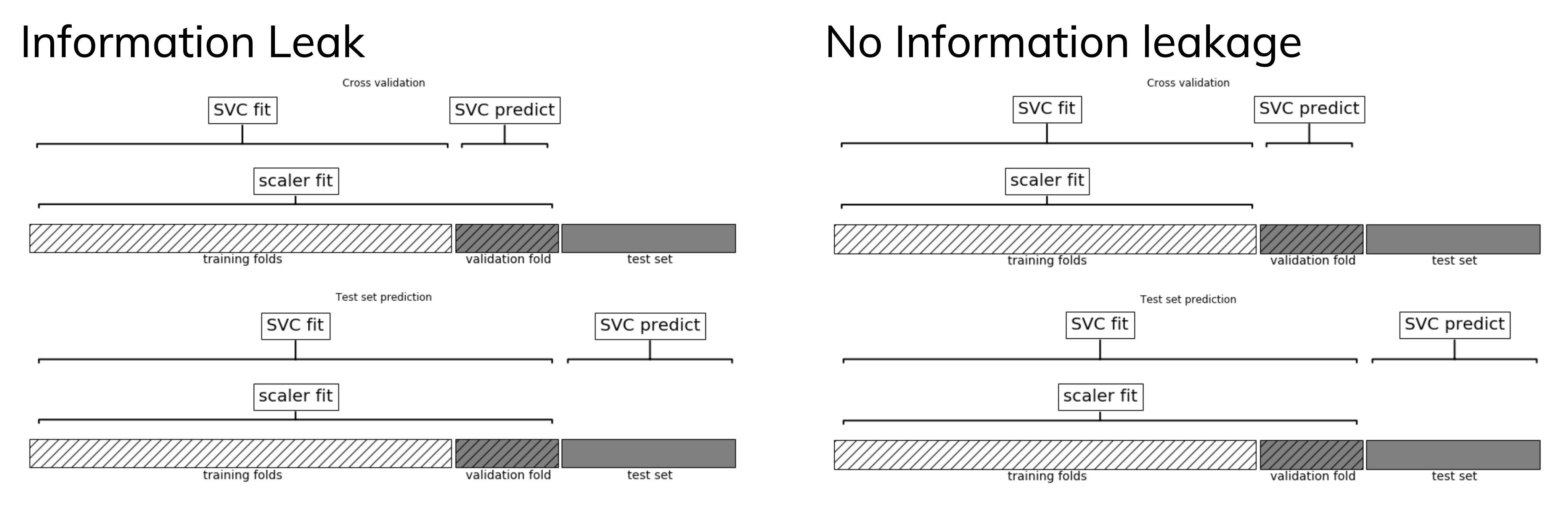
Data leakage
- Cross-validation: training set is split into training and validation sets for model selection
- Incorrect: Scaler is fit on whole training set before doing cross-validation
- Data leaks from validation folds into training folds, selected model may be optimistic
- Right: Scaler is fit on training folds only
Pipelines
- A pipeline is a combination of data transformation and learning algorithms
- It has a
fit,predict, andscoremethod, just like any other learning algorithm- Ensures that data transformations are applied correctly
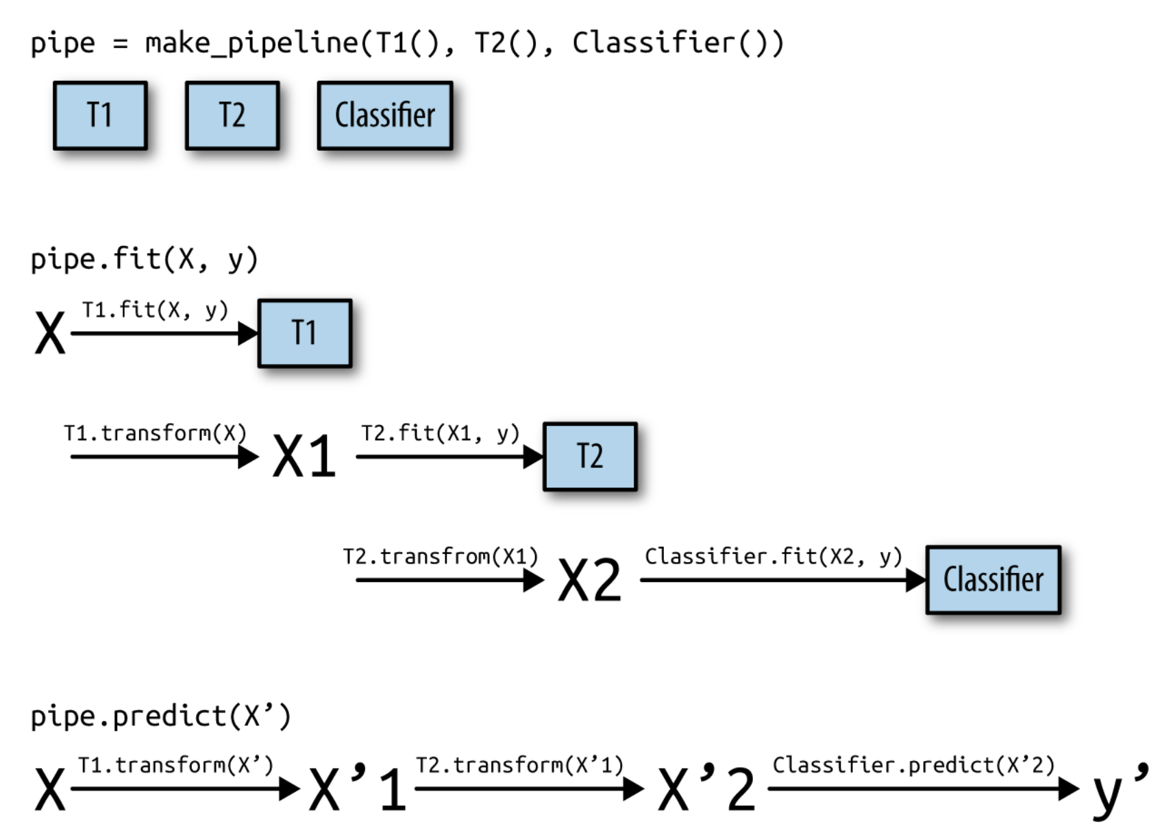
In practice (scikit-learn)
- A
pipelinecombines multiple processing steps in a single estimator - All but the last step should be data transformer (have a
transformmethod)
# Make pipeline, step names will be 'minmaxscaler' and 'linearsvc'
pipe = make_pipeline(MinMaxScaler(), LinearSVC())
# Build pipeline with named steps
pipe = Pipeline([("scaler", MinMaxScaler()), ("svm", LinearSVC())])

# Correct fit and score
score = pipe.fit(X_train, y_train).score(X_test, y_test)
# Retrieve trained model by name
svm = pipe.named_steps["svm"]
# Correct cross-validation
scores = cross_val_score(pipe, X, y)
- If you want to apply different preprocessors to different columns, use
ColumnTransformer - If you want to merge pipelines, you can use
FeatureUnionto concatenate columns
# 2 sub-pipelines, one for numeric features, other for categorical ones
numeric_pipe = make_pipeline(SimpleImputer(),StandardScaler())
categorical_pipe = make_pipeline(SimpleImputer(),OneHotEncoder())

# Using categorical pipe for features A,B,C, numeric pipe otherwise
preprocessor = make_column_transformer((categorical_pipe,
                                        ["A","B","C"]),
                                        remainder=numeric_pipe)

# Combine with learning algorithm in another pipeline
pipe = make_pipeline(preprocess, LinearSVC())
# Feature union of PCA features and selected features
union = FeatureUnion([("pca", PCA()), ("selected", SelectKBest())])
pipe = make_pipeline(union, LinearSVC())
ColumnTransformerconcatenates features in order
pipe = make_column_transformer((StandardScaler(),numeric_features),
                               (PCA(),numeric_features),
                               (OneHotEncoder(),categorical_features))
![]()
Pipeline selection
- We can safely use pipelines in model selection (e.g. grid search)
- Use
'__'to refer to the hyperparameters of a step, e.g.svm__C
# Correct grid search (can have hyperparameters of any step)
param_grid = {'svm__C': [0.001, 0.01],
              'svm__gamma': [0.001, 0.01, 0.1, 1, 10, 100]}
grid = GridSearchCV(pipe, param_grid=param_grid).fit(X,y)
# Best estimator is now the best pipeline
best_pipe = grid.best_estimator_

# Tune pipeline and evaluate on held-out test set
grid = GridSearchCV(pipe, param_grid=param_grid).fit(X_train,y_train)
grid.score(X_test,y_test)
Example: Tune multiple steps at once
pipe = make_pipeline(StandardScaler(),PolynomialFeatures(), Ridge())
param_grid = {'polynomialfeatures__degree': [1, 2, 3],
              'ridge__alpha': [0.001, 0.01, 0.1, 1, 10, 100]}
grid = GridSearchCV(pipe, param_grid=param_grid).fit(X_train, y_train)

Automatic Feature Selection
It can be a good idea to reduce the number of features to only the most useful ones
- Simpler models that generalize better (less overfitting)
- Curse of dimensionality (e.g. kNN)
- Even models such as RandomForest can benefit from this
- Sometimes it is one of the main methods to improve models (e.g. gene expression data)
- Faster prediction and training
- Training time can be quadratic (or cubic) in number of features
- Easier data collection, smaller models (less storage)
- More interpretable models: fewer features to look at
Example: bike sharing
- The Bike Sharing Demand dataset shows the amount of bikes rented in Washington DC
- Some features are clearly more informative than others (e.g. temp, hour)
- Some are correlated (e.g. temp and feel_temp)
- We add two random features at the end

Unsupervised feature selection
- Variance-based
- Remove (near) constant features
- Choose a small variance threshold
- Scale features before computing variance!
- Infrequent values may still be important
- Remove (near) constant features
- Covariance-based
- Remove correlated features
- The small differences may actually be important
- You don't know because you don't consider the target

Covariance based feature selection
- Remove features $X_i$ (= $\mathbf{X_{:,i}}$) that are highly correlated (have high correlation coefficient $\rho$) $$\rho (X_1,X_2)={\frac {{\mathrm {cov}}(X_1,X_2)}{\sigma (X_1)\sigma (X_2)}} = {\frac { \frac{1}{N-1} \sum_i (X_{i,1} - \overline{X_1})(X_{i,2} - \overline{X_2}) }{\sigma (X_1)\sigma (X_2)}}$$
- Should we remove
feel_temp? Ortemp? Maybe one correlates more with the target?

Supervised feature selection: overview
- Univariate: F-test and Mutual Information
- Model-based: Random Forests, Linear models, kNN
- Wrapping techniques (black-box search)
- Permutation importance
interactive(children=(Dropdown(description='method1', options=('FTest', 'MutualInformation', 'RandomForest', '…
Univariate statistics (F-test)
- Consider each feature individually (univariate), independent of the model that you aim to apply
- Use a statistical test: is there a linear statistically significant relationship with the target?
- Use F-statistic (or corresponding p value) to rank all features, then select features using a threshold
- Best $k$, best $k$ %, probability of removing useful features (FPR),...
- Cannot detect correlations (e.g. temp and feel_temp) or interactions (e.g. binary features)

F-statistic
- For regression: does feature $X_i$ correlate (positively or negatively) with the target $y$? $$\text{F-statistic} = \frac{\rho(X_i,y)^2}{1-\rho(X_i,y)^2} \cdot (N-1)$$
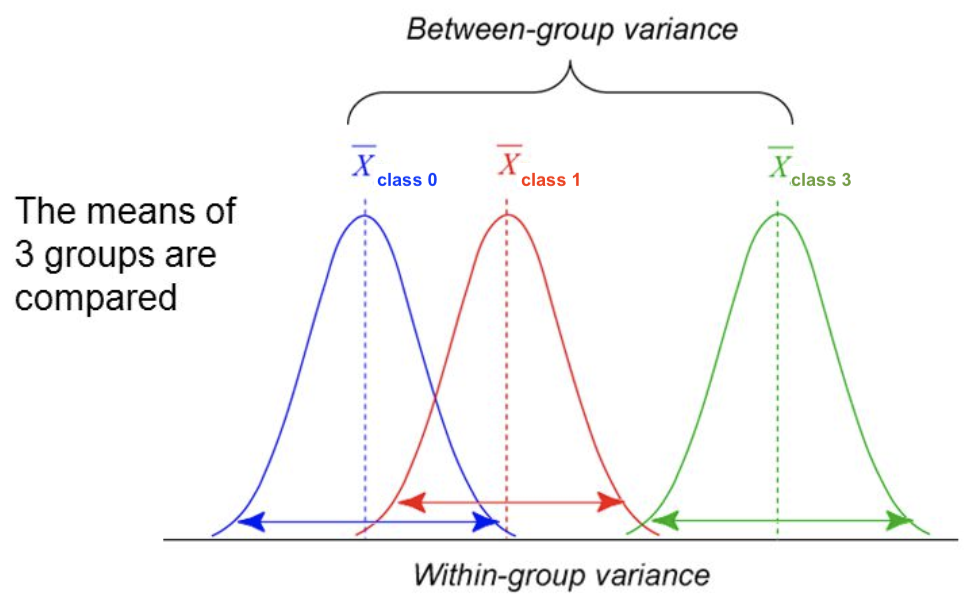
- For classification: uses ANOVA: does $X_i$ explain the between-class variance?
- Alternatively, use the $\chi^2$ test (only for categorical features)
$$\text{F-statistic} = \frac{\text{within-class variance}}{\text{between-class variance}} =\frac{var(\overline{X_i})}{\overline{var(X_i)}}$$
- Alternatively, use the $\chi^2$ test (only for categorical features)
$$\text{F-statistic} = \frac{\text{within-class variance}}{\text{between-class variance}} =\frac{var(\overline{X_i})}{\overline{var(X_i)}}$$
Mutual information
- Measures how much information $X_i$ gives about the target $Y$. In terms of entropy $H$: $$MI(X,Y) = H(X) + H(Y) - H(X,Y)$$
- Idea: estimate H(X) as the average distance between a data point and its $k$ Nearest Neighbors
- You need to choose $k$ and say which features are categorical
- Captures complex dependencies (e.g. hour, month), but requires more samples to be accurate

Model-based Feature Selection
- Use a tuned(!) supervised model to judge the importance of each feature
- Linear models (Ridge, Lasso, LinearSVM,...): features with highest weights (coefficients)
- Tree–based models: features used in first nodes (high information gain)
- Selection model can be different from the one you use for final modelling
- Captures interactions: features are more/less informative in combination (e.g. winter, temp)
- RandomForests: learns complex interactions (e.g. hour), but biased to high cardinality features

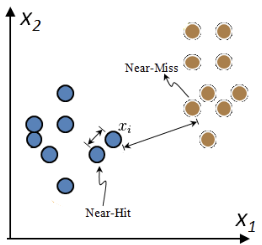
Relief: Model-based selection with kNN
- For I iterations, choose a random point $\mathbf{x_i}$ and find $k$ nearest neighbors $\mathbf{x_{k}}$
- Increase feature weights if $\mathbf{x_i}$ and $\mathbf{x_{k}}$ have different class (near miss), else decrease
- $\mathbf{w_i} = \mathbf{w_{i-1}} + (\mathbf{x_i} - \text{nearMiss}_i)^2 - (\mathbf{x_i} - \text{nearHit}_i)^2$
- Many variants: ReliefF (uses L1 norm, faster), RReliefF (for regression), ...
Iterative Model-based Feature Selection
- Dropping many features at once is not ideal: feature importance may change in subset
- Recursive Feature Elimination (RFE)
- Remove $s$ least important feature(s), recompute remaining importances, repeat
- Can be rather slow

Sequential feature selection (Wrapping)
- Evaluate your model with different sets of features, find best subset based on performance
- Greedy black-box search (can end up in local minima)
- Backward selection: remove least important feature, recompute importances, repeat
- Forward selection: set aside most important feature, recompute importances, repeat
- Floating: add best new feature, remove worst one, repeat (forward or backward)
- Stochastic search: use random mutations in candidate subset (e.g. simulated annealing)

Permutation feature importance
- Defined as the decrease in model performance when a single feature value is randomly shuffled
- This breaks the relationship between the feature and the target
- Model agnostic, metric agnostic, and can be calculated many times with different permutations
- Can be applied to unseen data (not possible with model-based techniques)
- Less biased towards high-cardinality features (compared with RandomForests)

Comparison
- Feature importances (scaled) and cross-validated $R^2$ score of pipeline
- Pipeline contains features selection + Ridge
- Selection threshold value ranges from 25% to 100% of all features
- Best method ultimately depends on the problem and dataset at hand
interactive(children=(Dropdown(description='method1', options=('FTest', 'MutualInformation', 'RandomForest', '…

In practice (scikit-learn)
- Unsupervised:
VarianceTreshold
selector = VarianceThreshold(threshold=0.01)
X_selected = selector.fit_transform(X)
variances = selector.variances_
- Univariate:
- For regression:
f_regression,mutual_info_regression - For classification:
f_classification,chi2,mutual_info_classication - Selecting:
SelectKBest,SelectPercentile,SelectFpr,...
- For regression:
selector = SelectPercentile(score_func=f_regression, percentile=50)
X_selected = selector.fit_transform(X,y)
selected_features = selector.get_support()
f_values, p_values = f_regression(X,y)
mi_values = mutual_info_regression(X,y,discrete_features=[])
- Model-based:
SelectFromModel: requires a model and a selection thresholdRFE,RFECV(recursive feature elimination): requires model and final nr features
selector = SelectFromModel(RandomForestRegressor(), threshold='mean')
rfe_selector = RFE(RidgeCV(), n_features_to_select=20)
X_selected = selector.fit_transform(X)
rf_importances = Randomforest().fit(X, y).feature_importances_
- Sequential feature selection (from
mlxtend, sklearn-compatible)
selector = SequentialFeatureSelector(RidgeCV(), k_features=20, forward=True,
                                     floating=True)
X_selected = selector.fit_transform(X)
- Permutation Importance (in
sklearn.inspection), no fit-transform interface
importances = permutation_importance(RandomForestRegressor().fit(X,y),
                                     X, y, n_repeats=10).importances_mean
feature_ids = (-importances).argsort()[:n]
Feature Engineering
- Create new features based on existing ones
- Polynomial features
- Interaction features
- Binning
- Mainly useful for simple models (e.g. linear models)
- Other models can learn interations themselves
- But may be slower, less robust than linear models
Polynomials
- Add all polynomials up to degree $d$ and all products
- Equivalent to polynomial basis expansions $$[1, x_1, ..., x_p] \xrightarrow{} [1, x_1, ..., x_p, x_1^2, ..., x_p^2, ..., x_p^d, x_1 x_2, ..., x_{p-1} x_p]$$

Binning
- Partition numeric feature values into $n$ intervals (bins)
- Create $n$ new one-hot features, 1 if original value falls in corresponding bin
- Models different intervals differently (e.g. different age groups)
| orig | [-3.0,-1.5] | [-1.5,0.0] | [0.0,1.5] | [1.5,3.0] | |
|---|---|---|---|---|---|
| 0 | -0.752759 | 0.000000 | 1.000000 | 0.000000 | 0.000000 |
| 1 | 2.704286 | 0.000000 | 0.000000 | 0.000000 | 1.000000 |
| 2 | 1.391964 | 0.000000 | 0.000000 | 1.000000 | 0.000000 |

Binning + interaction features
- Add interaction features (or product features )
- Product of the bin encoding and the original feature value
- Learn different weights per bin
| orig | b0 | b1 | b2 | b3 | X*b0 | X*b1 | X*b2 | X*b3 | |
|---|---|---|---|---|---|---|---|---|---|
| 0 | -0.752759 | 0.000000 | 1.000000 | 0.000000 | 0.000000 | -0.000000 | -0.752759 | -0.000000 | -0.000000 |
| 1 | 2.704286 | 0.000000 | 0.000000 | 0.000000 | 1.000000 | 0.000000 | 0.000000 | 0.000000 | 2.704286 |
| 2 | 1.391964 | 0.000000 | 0.000000 | 1.000000 | 0.000000 | 0.000000 | 0.000000 | 1.391964 | 0.000000 |

Categorical feature interactions
- One-hot-encode categorical feature
- Multiply every one-hot-encoded column with every numeric feature
- Allows to built different submodels for different categories
| gender | age | pageviews | time | |
|---|---|---|---|---|
| 0 | M | 14 | 70 | 269 |
| 1 | F | 16 | 12 | 1522 |
| 2 | M | 12 | 42 | 235 |
| 3 | F | 25 | 64 | 63 |
| 4 | F | 22 | 93 | 21 |
| age_M | pageviews_M | time_M | gender_M_M | age_F | pageviews_F | time_F | gender_F_F | |
|---|---|---|---|---|---|---|---|---|
| 0 | 14 | 70 | 269 | 1 | 0 | 0 | 0 | 0 |
| 1 | 0 | 0 | 0 | 0 | 16 | 12 | 1522 | 1 |
| 2 | 12 | 42 | 235 | 1 | 0 | 0 | 0 | 0 |
| 3 | 0 | 0 | 0 | 0 | 25 | 64 | 63 | 1 |
| 4 | 0 | 0 | 0 | 0 | 22 | 93 | 21 | 1 |
Missing value imputation
- Data can be missing in different ways:
- Missing Completely at Random (MCAR): purely random points are missing
- Missing at Random (MAR): something affects missingness, but no relation with the value
- E.g. faulty sensors, some people don't fill out forms correctly
- Missing Not At Random (MNAR): systematic missingness linked to the value
- Has to be modelled or resolved (e.g. sensor decay, sick people leaving study)
- Missingness can be encoded in different ways:'?', '-1', 'unknown', 'NA',...
- Also labels can be missing (remove example or use semi-supervised learning)
Overview
- Mean/constant imputation
- kNN-based imputation
- Iterative (model-based) imputation
- Matrix Factorization techniques
interactive(children=(Dropdown(description='imputer', options=('Mean Imputation', 'kNN Imputation', 'Iterative…

Mean imputation
- Replace all missing values of a feature by the same value
- Numerical features: mean or median
- Categorical features: most frequent category
- Constant value, e.g. 0 or 'missing' for text features
- Optional: add an indicator column for missingness
- Example: Iris dataset (randomly removed values in 3rd and 4th column)

kNN imputation
- Use special version of kNN to predict value of missing points
- Uses only non-missing data when computing distances
Iterative (model-based) Imputation
- Better known as Multiple Imputation by Chained Equations (MICE)
- Iterative approach
- Do first imputation (e.g. mean imputation)
- Train model (e.g. RandomForest) to predict missing values of a given feature
- Train new model on imputed data to predict missing values of the next feature
- Repeat $m$ times in round-robin fashion, leave one feature out at a time

Matrix Factorization
- Basic idea: low-rank approximation
- Replace missing values by 0
- Factorize $\mathbf{X}$ with rank $r$: $\mathbf{X}^{n\times p}=\mathbf{U}^{n\times r} \mathbf{V}^{r\times p}$
- With n data points and p features
- Solved using gradient descent
- Recompute $\mathbf{X}$: now complete

Soft-thresholded Singular Value Decomposition (SVD)
- Same basic idea, but smoother
- Replace missing values by 0, compute SVD: $\mathbf{X}=\mathbf{U} \mathbf{\Sigma} \mathbf{V^{T}}$
- Solved with gradient descent
- Reduce eigenvalues by shrinkage factor: $\lambda_i = s\cdot\lambda_i$
- Recompute $\mathbf{X}$: now complete
- Repeat for $m$ iterations
- Replace missing values by 0, compute SVD: $\mathbf{X}=\mathbf{U} \mathbf{\Sigma} \mathbf{V^{T}}$

Comparison
- Best method depends on the problem and dataset at hand. Use cross-validation.
- Iterative Imputation (MICE) generally works well for missing (completely) at random data
- Can be slow if the prediction model is slow
- Low-rank approximation techniques scale well to large datasets
interactive(children=(Dropdown(description='imputer', options=('Mean Imputation', 'kNN Imputation', 'Iterative…
In practice (scikit-learn)
- Simple replacement:
SimpleImputer- Strategies:
mean(numeric),median,most_frequent(categorical) - Choose whether to add indicator columns, and how missing values are encoded
- Strategies:
imp = SimpleImputer(strategy='mean', missing_values=np.nan, add_indicator=False)
X_complete = imp.fit_transform(X_train)
- kNN Imputation:
KNNImputer
imp = KNNImputer(n_neighbors=5)
X_complete = imp.fit_transform(X_train)
- Multiple Imputation (MICE):
IterativeImputer- Choose estimator (default:
BayesianRidge) and number of iterations (default 10)
- Choose estimator (default:
imp = IterativeImputer(estimator=RandomForestClassifier(), max_iter=10)
X_complete = imp.fit_transform(X_train)
In practice (fancyimpute)
- Cannot be used in CV pipelines (has
fit_transformbut notransform) - Soft-Thresholded SVD:
SoftImpute- Choose max number of gradient descent iterations
- Choose shrinkage value for eigenvectors (default: $\frac{1}{N}$)
imp = SoftImpute(max_iter=10, shrinkage_value=None)
X_complete = imp.fit_transform(X)
- Low-rank imputation:
MatrixFactorization- Choose rank of the low-rank approximation
- Gradient descent hyperparameters: learning rate, epochs,...
- Several variants exist
imp = MatrixFactorization(rank=10, learning_rate=0.001, epochs=10000)
X_complete = imp.fit_transform(X)
Handling imbalanced data
- Problem:
- You have a majority class with many times the number of examples as the minority class
- Or: classes are balanced, but associated costs are not (e.g. FN are worse than FP)
- We already covered some ways to resolve this:
- Add class weights to the loss function: give the minority class more weight
- In practice: set
class_weight='balanced'
- In practice: set
- Change the prediction threshold to minimize false negatives or false positives
- Add class weights to the loss function: give the minority class more weight
- There are also things we can do by preprocessing the data
- Resample the data to correct the imbalance
- Random or model-based
- Generate synthetic samples for the minority class
- Build ensembles over different resampled datasets
- Combinations of these
- Resample the data to correct the imbalance
Random Undersampling
- Copy the points from the minority class
- Randomly sample from the majority class (with or without replacement) until balanced
- Optionally, sample until a certain imbalance ratio (e.g. 1/5) is reached
- Multi-class: repeat with every other class
- Preferred for large datasets, often yields smaller/faster models with similar performance

Model-based Undersampling
- Edited Nearest Neighbors
- Remove all majority samples that are misclassified by kNN (mode) or that have a neighbor from the other class (all).
- Remove their influence on the minority samples
- Condensed Nearest Neighbors
- Remove all majority samples that are not misclassified by kNN
- Focus on only the hard samples

Random Oversampling
- Copy the points from the majority class
- Randomly sample from the minority class, with replacement, until balanced
- Optionally, sample until a certain imbalance ratio (e.g. 1/5) is reached
- Makes models more expensive to train, doens't always improve performance
- Similar to giving minority class(es) a higher weight (and more expensive)

Synthetic Minority Oversampling Technique (SMOTE)
- Repeatedly choose a random minority point and a neighboring minority point
- Pick a new, artificial point on the line between them (uniformly)
- May bias the data. Be careful never to create artificial points in the test set.
- ADASYN (Adaptive Synthetic)
- Similar, but starts from 'hard' minority points (misclassified by kNN)

Combined techniques
- Combines over- and under-sampling
- E.g. oversampling with SMOTE, undersampling with Edited Nearest Neighbors (ENN)
- SMOTE can generate 'noisy' point, close to majority class points
- ENN will remove up these majority points to 'clean up' the space

Ensemble Resampling
- Bagged ensemble of balanced base learners. Acts as a learner, not a preprocessor
- BalancedBagging: take bootstraps, randomly undersample each, train models (e.g. trees)
- Benefits of random undersampling without throwing out so much data
- Easy Ensemble: take multiple random undersamplings directly, train models
- Traditionally uses AdaBoost as base learner, but can be replaced

Comparison
- The best method depends on the data (amount of data, imbalance,...)
- For a very large dataset, random undersampling may be fine
- You still need to choose the appropriate learning algorithms
- Don't forget about class weighting and prediction thresholding
- Some combinations are useful, e.g. SMOTE + class weighting + thresholding
interactive(children=(Dropdown(description='sampler', options=(RandomUnderSampler(), EditedNearestNeighbours()…

In practice (imblearn)
- Follows fit-sample paradigm (equivalent of fit-transform, but also affects y)
- Undersampling: RandomUnderSampler, EditedNearestNeighbours,...
- (Synthetic) Oversampling: RandomOverSampler, SMOTE, ADASYN,...
- Combinations: SMOTEENN,...
X_resampled, y_resampled = SMOTE(k_neighbors=5).fit_sample(X, y)
- Can be used in imblearn pipelines (not sklearn pipelines)
- imblearn pipelines are compatible with GridSearchCV,...
- Sampling is only done in
fit(not inpredict)
smote_pipe = make_pipeline(SMOTE(), LogisticRegression())
scores = cross_validate(smote_pipe, X_train, y_train)
param_grid = {"k_neighbors": [3,5,7]}
grid = GridSearchCV(smote_pipe, param_grid=param_grid, X, y)
- The ensembling techniques should be used as wrappers
clf = EasyEnsembleClassifier(base_estimator=SVC()).fit(X_train, y_train)
Real-world data
- The effect of sampling procedures can be unpredictable
- Best method can depend on the data and FP/FN trade-offs
- SMOTE and ensembling techniques often work well
interactive(children=(Dropdown(description='dataset', options=('Speech', 'mc1', 'mammography'), value='Speech'…

Summary
- Data preprocessing is a crucial part of machine learning
- Scaling is important for many distance-based methods (e.g. kNN, SVM, Neural Nets)
- Categorical encoding is necessary for numeric methods (or implementations)
- Selecting features can speed up models and reduce overfitting
- Feature engineering is often useful for linear models
- It is often better to impute missing data than to remove data
- Imbalanced datasets require extra care to build useful models
- Pipelines allow us to encapsulate multiple steps in a convenient way
- Avoids data leakage, crucial for proper evaluation
- Choose the right preprocessing steps and models in your pipeline
- Cross-validation helps, but the search space is huge
- Smarter techniques exist to automate this process (AutoML)