Lecture 5. Ensemble Learning¶

Crowd intelligence

Joaquin Vanschoren

Ensemble learning¶

If different models make different mistakes, can we simply average the predictions?
Voting Classifier: gives every model a vote on the class label
- Hard vote: majority class wins (class order breaks ties)
- Soft vote: sum class probabilities $p_{m,c}$ over $M$ models: $\underset{c}{\operatorname{argmax}} \sum_{m=1}^{M} w_c p_{m,c}$
- Classes can get different weights $w_c$ (default: $w_c=1$)

interactive(children=(Dropdown(description='model1', options=(LogisticRegression(C=100), DecisionTreeClassifie…

Why does this work?
- Different models may be good at different 'parts' of data (even if they underfit)
- Individual mistakes can be 'averaged out' (especially if models overfit)
Which models should be combined?
Bias-variance analysis teaches us that we have two options:
- If model underfits (high bias, low variance): combine with other low-variance models
  - Need to be different: 'experts' on different parts of the data
  - Bias reduction. Can be done with Boosting
- If model overfits (low bias, high variance): combine with other low-bias models
  - Need to be different: individual mistakes must be different
  - Variance reduction. Can be done with Bagging
Models must be uncorrelated but good enough (otherwise the ensemble is worse)
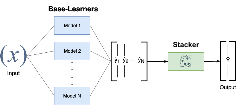
We can also learn how to combine the predictions of different models: Stacking

Decision trees (recap)¶

Representation: Tree that splits data points into leaves based on tests
Evaluation (loss): Heuristic for purity of leaves (Gini index, entropy,...)
Optimization: Recursive, heuristic greedy search (Hunt's algorithm)
- Consider all splits (thresholds) between adjacent data points, for every feature
- Choose the one that yields the purest leafs, repeat

interactive(children=(IntSlider(value=3, description='depth', max=5, min=1), Output()), _dom_classes=('widget-…

Evaluation (loss function for classification)¶

Every leaf predicts a class probability $\hat{p}_c$ = the relative frequency of class $c$
Leaf impurity measures (splitting criteria) for $L$ leafs, leaf $l$ has data $X_l$:
- Gini-Index: $Gini(X_{l}) = \sum_{c\neq c'} \hat{p}_c \hat{p}_{c'}$
- Entropy (more expensive): $E(X_{l}) = -\sum_{c\neq c'} \hat{p}_c \log_{2}\hat{p}_c$
- Best split maximizes information gain (idem for Gini index) $$ Gain(X,X_i) = E(X) - \sum_{l=1}^L \frac{|X_{i=l}|}{|X_{i}|} E(X_{i=l}) $$

Regression trees¶

Every leaf predicts the mean target value $\mu$ of all points in that leaf
Choose the split that minimizes squared error of the leaves: $\sum_{x_{i} \in L} (y_i - \mu)^2$
Yields non-smooth step-wise predictions, cannot extrapolate

Impurity/Entropy-based feature importance¶

We can measure the importance of features (to the model) based on
- Which features we split on
- How high up in the tree we split on them (first splits ar emore important)

Under- and overfitting¶

We can easily control the (maximum) depth of the trees as a hyperparameter
Bias-variance analysis:
- Shallow trees have high bias but very low variance (underfitting)
- Deep trees have high variance but low bias (overfitting)
Because we can easily control their complexity, they are ideal for ensembling
- Deep trees: keep low bias, reduce variance with Bagging
- Shallow trees: keep low variance, reduce bias with Boosting

Bagging (Bootstrap Aggregating)¶

Obtain different models by training the same model on different training samples
- Reduce overfitting by averaging out individual predictions (variance reduction)
In practice: take $I$ bootstrap samples of your data, train a model on each bootstrap
- Higher $I$: more models, more smoothing (but slower training and prediction)
Base models should be unstable: different training samples yield different models
- E.g. very deep decision trees, or even randomized decision trees
- Deep Neural Networks can also benefit from bagging (deep ensembles)
Prediction by averaging predictions of base models
- Soft voting for classification (possibly weighted)
- Mean value for regression
Can produce uncertainty estimates as well
- By combining class probabilities of individual models (or variances for regression)

Random Forests¶

Uses randomized trees to make models even less correlated (more unstable)
- At every split, only consider max_features features, randomly selected
Extremely randomized trees: considers 1 random threshold for random set of features (faster)

interactive(children=(Dropdown(description='model', options=(RandomForestClassifier(n_estimators=5, n_jobs=-1,…

Effect on bias and variance¶

Increasing the number of models (trees) decreases variance (less overfitting)
Bias is mostly unaffected, but will increase if the forest becomes too large (oversmoothing)

In practice¶

Different implementations can be used. E.g. in scikit-learn:
- BaggingClassifier: Choose your own base model and sampling procedure
- RandomForestClassifier: Default implementation, many options
- ExtraTreesClassifier: Uses extremely randomized trees
Most important parameters:
- n_estimators (>100, higher is better, but diminishing returns)
  - Will start to underfit (bias error component increases slightly)
- max_features
  - Defaults: $sqrt(p)$ for classification, $log2(p)$ for regression
  - Set smaller to reduce space/time requirements
- parameters of trees, e.g. max_depth, min_samples_split,...
  - Prepruning useful to reduce model size, but don't overdo it
Easy to parallelize (set n_jobs to -1)
Fix random_state (bootstrap samples) for reproducibility

Out-of-bag error¶

RandomForests don't need cross-validation: you can use the out-of-bag (OOB) error
For each tree grown, about 33% of samples are out-of-bag (OOB)
- Remember which are OOB samples for every model, do voting over these
OOB error estimates are great to speed up model selection
- As good as CV estimates, althought slightly pessimistic
In scikit-learn: oob_error = 1 - clf.oob_score_

Feature importance¶

RandomForests provide more reliable feature importances, based on many alternative hypotheses (trees)

Other tips¶

Model calibration
- RandomForests are poorly calibrated.
- Calibrate afterwards (e.g. isotonic regression) if you aim to use probabilities
Warm starting
- Given an ensemble trained for $I$ iterations, you can simply add more models later
- You warm start from the existing model instead of re-starting from scratch
- Can be useful to train models on new, closely related data
  - Not ideal if the data batches change over time (concept drift)
  - Boosting is more robust against this (see later)

Strength and weaknesses¶

RandomForest are among most widely used algorithms:
- Don't require a lot of tuning
- Typically very accurate
- Handles heterogeneous features well (trees)
- Implictly selects most relevant features
Downsides:
- less interpretable, slower to train (but parallellizable)
- don't work well on high dimensional sparse data (e.g. text)

Adaptive Boosting (AdaBoost)¶

Obtain different models by reweighting the training data every iteration
- Reduce underfitting by focusing on the 'hard' training examples
Increase weights of instances misclassified by the ensemble, and vice versa
Base models should be simple so that different instance weights lead to different models
- Underfitting models: decision stumps (or very shallow trees)
- Each is an 'expert' on some parts of the data
Additive model: Predictions at iteration $I$ are sum of base model predictions
- In Adaboost, also the models each get a unique weight $w_i$ $$f_I(\mathbf{x}) = \sum_{i=1}^I w_i g_i(\mathbf{x})$$
Adaboost minimizes exponential loss. For instance-weighted error $\varepsilon$: $$\mathcal{L}_{Exp} = \sum_{n=1}^N e^{\varepsilon(f_I(\mathbf{x}))}$$
By deriving $\frac{\partial \mathcal{L}}{\partial w_i}$ you can find that optimal $w_{i} = \frac{1}{2}\log(\frac{1-\varepsilon}{\varepsilon})$

AdaBoost algorithm¶

Initialize sample weights: $s_{n,0} = \frac{1}{N}$
Build a model (e.g. decision stumps) using these sample weights
Give the model a weight $w_i$ related to its weighted error rate $\varepsilon$ $$w_{i} = \lambda\log(\frac{1-\varepsilon}{\varepsilon})$$
- Good trees get more weight than bad trees
- Logit function maps error $\varepsilon$ from [0,1] to weight in [-Inf,Inf] (use small minimum error)
- Learning rate $\lambda$ (shrinkage) decreases impact of individual classifiers
  - Small updates are often better but requires more iterations
Update the sample weights
- Increase weight of incorrectly predicted samples: $s_{n,i+1} = s_{n,i}e^{w_i}$
- Decrease weight of correctly predicted samples: $s_{n,i+1} = s_{n,i}e^{-w_i}$
- Normalize weights to add up to 1
Repeat for $I$ iterations

AdaBoost variants¶

Discrete Adaboost: error rate $\varepsilon$ is simply the error rate (1-Accuracy)
Real Adaboost: $\varepsilon$ is based on predicted class probabilities $\hat{p}_c$ (better)
AdaBoost for regression: $\varepsilon$ is either linear ($|y_i-\hat{y}_i|$), squared ($(y_i-\hat{y}_i)^2$), or exponential loss
GentleBoost: adds a bound on model weights $w_i$
LogitBoost: Minimizes logistic loss instead of exponential loss $$\mathcal{L}_{Logistic} = \sum_{n=1}^N log(1+e^{\varepsilon(f_I(\mathbf{x}))})$$

Adaboost in action¶

Size of the samples represents sample weight
Background shows the latest tree's predictions

interactive(children=(IntSlider(value=30, description='iteration', max=60), Output()), _dom_classes=('widget-i…

Examples¶

Bias-Variance analysis¶

AdaBoost reduces bias (and a little variance)
- Boosting is a bias reduction technique
Boosting too much will eventually increase variance

Gradient Boosting¶

Ensemble of models, each fixing the remaining mistakes of the previous ones
- Each iteration, the task is to predict the residual error of the ensemble
Additive model: Predictions at iteration $I$ are sum of base model predictions
- Learning rate (or shrinkage ) $\eta$: small updates work better (reduces variance) $$f_I(\mathbf{x}) = g_0(\mathbf{x}) + \sum_{i=1}^I \eta \cdot g_i(\mathbf{x}) = f_{I-1}(\mathbf{x}) + \eta \cdot g_I(\mathbf{x})$$
The pseudo-residuals $r_i$ are computed according to differentiable loss function
- E.g. least squares loss for regression and log loss for classification
- Gradient descent: predictions get updated step by step until convergence $$g_i(\mathbf{x}) \approx r_{i} = - \frac{\partial \mathcal{L}(y_i,f_{i-1}(x_i))}{\partial f_{i-1}(x_i)}$$
Base models $g_i$ should be low variance, but flexible enough to predict residuals accurately
- E.g. decision trees of depth 2-5

Gradient Boosting Trees (Regression)¶

Base models are regression trees, loss function is square loss: $\mathcal{L} = \frac{1}{2}(y_i - \hat{y}_i)^2$
The pseudo-residuals are simply the prediction errors for every sample: $$r_i = -\frac{\partial \mathcal{L}}{\partial \hat{y}} = -2 * \frac{1}{2}(y_i - \hat{y}_i) * (-1) = y_i - \hat{y}_i$$
Initial model $g_0$ simply predicts the mean of $y$
For iteration $m=1..M$:
- For all samples i=1..n, compute pseudo-residuals $r_i = y_i - \hat{y}_i$
- Fit a new regression tree model $g_m(\mathbf{x})$ to $r_{i}$
  - In $g_m(\mathbf{x})$, each leaf predicts the mean of all its values
- Update ensemble predictions $\hat{y} = g_0(\mathbf{x}) + \sum_{m=1}^M \eta \cdot g_m(\mathbf{x})$
Early stopping (optional): stop when performance on validation set does not improve for $nr$ iterations

Gradient Boosting Regression in action¶

Residuals quickly drop to (near) zero

interactive(children=(IntSlider(value=30, description='step', max=60), Output()), _dom_classes=('widget-intera…

GradientBoosting Algorithm (Classification)¶

Base models are regression trees, predict probability of positive class $p$
- For multi-class problems, train one tree per class
Use (binary) log loss, with true class $y_i \in {0,1}$: $\mathcal{L_{log}} = - \sum_{i=1}^{N} \big[ y_i log(p_i) + (1-y_i) log(1-p_i) \big] $
The pseudo-residuals are simply the difference between true class and predicted $p$: $$\frac{\partial \mathcal{L}}{\partial \hat{y}} = \frac{\partial \mathcal{L}}{\partial log(p_i)} = y_i - p_i$$
Initial model $g_0$ predicts $p = log(\frac{\#positives}{\#negatives})$
For iteration $m=1..M$:
- For all samples i=1..n, compute pseudo-residuals $r_i = y_i - p_i$
- Fit a new regression tree model $g_m(\mathbf{x})$ to $r_{i}$
  - In $g_m(\mathbf{x})$, each leaf predicts $\frac{\sum_{i} r_i}{\sum_{i} p_i(1-p_i)}$
- Update ensemble predictions $\hat{y} = g_0(\mathbf{x}) + \sum_{m=1}^M \eta \cdot g_m(\mathbf{x})$
Early stopping (optional): stop when performance on validation set does not improve for $nr$ iterations

Gradient Boosting Classification in action¶

Size of the samples represents the residual weights: most quickly drop to (near) zero

interactive(children=(IntSlider(value=30, description='iteration', max=60, min=1), Output()), _dom_classes=('w…

Examples¶

Bias-variance analysis¶

Gradient Boosting is very effective at reducing bias error
Boosting too much will eventually increase variance

Feature importance¶

Gradient Boosting also provide feature importances, based on many trees
Compared to RandomForests, the trees are smaller, hence more features have zero importance

Gradient Boosting: strengths and weaknesses¶

Among the most powerful and widely used models
Work well on heterogeneous features and different scales
Typically better than random forests, but requires more tuning, longer training
Does not work well on high-dimensional sparse data

Main hyperparameters:

n_estimators: Higher is better, but will start to overfit
learning_rate: Lower rates mean more trees are needed to get more complex models
- Set n_estimators as high as possible, then tune learning_rate
- Or, choose a learning_rate and use early stopping to avoid overfitting
max_depth: typically kept low (<5), reduce when overfitting
max_features: can also be tuned, similar to random forests
n_iter_no_change: early stopping: algorithm stops if improvement is less than a certain tolerance tol for more than n_iter_no_change iterations.

Extreme Gradient Boosting (XGBoost)¶

Faster version of gradient boosting: allows more iterations on larger datasets
Normal regression trees: split to minimize squared loss of leaf predictions
- XGBoost trees only fit residuals: split so that residuals in leaf are more similar
Don't evaluate every split point, only $q$ quantiles per feature (binning)
- $q$ is hyperparameter (sketch_eps, default 0.03)
For large datasets, XGBoost uses approximate quantiles
- Can be parallelized (multicore) by chunking the data and combining histograms of data
- For classification, the quantiles are weighted by $p(1-p)$
Gradient descent sped up by using the second derivative of the loss function
Strong regularization by pre-pruning the trees
Column and row are randomly subsampled when computing splits
Support for out-of-core computation (data compression in RAM, sharding,...)

XGBoost in practice¶

Not part of scikit-learn, but HistGradientBoostingClassifier is similar
- binning, multicore,...
The xgboost python package is sklearn-compatible
- Install separately, conda install -c conda-forge xgboost
- Allows learning curve plotting and warm-starting
Further reading:

LightGBM¶

Another fast boosting technique

Uses gradient-based sampling
- use all instances with large gradients/residuals (e.g. 10% largest)
- randomly sample instances with small gradients, ignore the rest
- intuition: samples with small gradients are already well-trained.
- requires adapted information gain criterion
Does smarter encoding of categorical features

CatBoost¶

Another fast boosting technique

Optimized for categorical variables
- Uses bagged and smoothed version of target encoding
Uses symmetric trees: same split for all nodes on a given level aka
- Can be much faster
Allows monotonicity constraints for numeric features
- Model must be be a non-decreasing function of these features
Lots of tooling (e.g. GPU training)

Stacking¶

Choose $M$ different base-models, generate predictions
Stacker (meta-model) learns mapping between predictions and correct label
- Can also be repeated: multi-level stacking
- Popular stackers: linear models (fast) and gradient boosting (accurate)
Cascade stacking: adds base-model predictions as extra features
Models need to be sufficiently different, be experts at different parts of the data
Can be very accurate, but also very slow to predict

Other ensembling techniques¶

Hyper-ensembles: same basic model but with different hyperparameter settings
- Can combine overfitted and underfitted models
Deep ensembles: ensembles of deep learning models
Bayes optimal classifier: ensemble of all possible models (largely theoretic)
Bayesian model averaging: weighted average of probabilistic models, weighted by their posterior probabilities
Cross-validation selection: does internal cross-validation to select best of $M$ models
Any combination of different ensembling techniques

Algorithm overview¶

Name	Representation	Loss function	Optimization	Regularization
Classification trees	Decision tree	Entropy / Gini index	Hunt's algorithm	Tree depth,...
Regression trees	Decision tree	Square loss	Hunt's algorithm	Tree depth,...
RandomForest	Ensemble of randomized trees	Entropy / Gini / Square	(Bagging)	Number/depth of trees,...
AdaBoost	Ensemble of stumps	Exponential loss	Greedy search	Number/depth of trees,...
GradientBoostingRegression	Ensemble of regression trees	Square loss	Gradient descent	Number/depth of trees,...
GradientBoostingClassification	Ensemble of regression trees	Log loss	Gradient descent	Number/depth of trees,...
XGBoost, LightGBM, CatBoost	Ensemble of XGBoost trees	Square/log loss	2nd order gradients	Number/depth of trees,...
Stacking	Ensemble of heterogeneous models	/	/	Number of models,...

Summary¶

Ensembles of voting classifiers improve performance
- Which models to choose? Consider bias-variance tradeoffs!
Bagging / RandomForest is a variance-reduction technique
- Build many high-variance (overfitting) models on random data samples
  - The more different the models, the better
- Aggregation (soft voting) over many models reduces variance
  - Diminishing returns, over-smoothing may increase bias error
- Parallellizes easily, doesn't require much tuning
Boosting is a bias-reduction technique
- Build low-variance models that correct each other's mistakes
  - By reweighting misclassified samples: AdaBoost
  - By predicting the residual error: Gradient Boosting
- Additive models: predictions are sum of base-model predictions
  - Can drive the error to zero, but risk overfitting
- Doesn't parallelize easily. Slower to train, much faster to predict.
  - XGBoost,LightGBM,... are fast and offer some parallellization
Stacking: learn how to combine base-model predictions
- Base-models still have to be sufficiently different