Lecture 3: Kernelization

Making linear models non-linear

Joaquin Vanschoren

Feature Maps

• Linear models: $\hat{y} = \mathbf{w}\mathbf{x} + w_0 = \sum_{i=1}^{p} w_i x_i + w_0 = w_0 + w_1 x_1 + ... + w_p x_p $

• When we cannot fit the data well, we can add non-linear transformations of the features

• Feature map (or basis expansion ) $\phi$ : $ X \rightarrow \mathbb{R}^d $

$$y=\textbf{w}^T\textbf{x} \rightarrow y=\textbf{w}^T\phi(\textbf{x})$$

• E.g. Polynomial feature map: all polynomials up to degree $d$ and all products

$$[1, x_1, ..., x_p] \xrightarrow{\phi} [1, x_1, ..., x_p, x_1^2, ..., x_p^2, ..., x_p^d, x_1 x_2, ..., x_{p-1} x_p]$$

• Example with $p=1, d=3$ :

$$y=w_0 + w_1 x_1 \xrightarrow{\phi} y=w_0 + w_1 x_1 + w_2 x_1^2 + w_3 x_1^3$$

Ridge regression example

Weights: [0.418]

• Add all polynomials $x^d$ up to degree 10 and fit again:
  • e.g. use sklearn PolynomialFeatures

	x0	x0^2	x0^3	x0^4	x0^5	x0^6	x0^7	x0^8	x0^9	x0^10
0	-0.752759	0.566647	-0.426548	0.321088	-0.241702	0.181944	-0.136960	0.103098	-0.077608	0.058420
1	2.704286	7.313162	19.776880	53.482337	144.631526	391.124988	1057.713767	2860.360362	7735.232021	20918.278410
2	1.391964	1.937563	2.697017	3.754150	5.225640	7.273901	10.125005	14.093639	19.617834	27.307312
3	0.591951	0.350406	0.207423	0.122784	0.072682	0.043024	0.025468	0.015076	0.008924	0.005283
4	-2.063888	4.259634	-8.791409	18.144485	-37.448187	77.288869	-159.515582	329.222321	-679.478050	1402.366700

Weights: [ 0.643  0.297 -0.69  -0.264  0.41   0.096 -0.076 -0.014  0.004  0.001]

How expensive is this?

• You may need MANY dimensions to fit the data
  • Memory and computational cost
  • More weights to learn, more likely overfitting

• Ridge has a closed-form solution which we can compute with linear algebra: $$w^{*} = (X^{T}X + \alpha I)^{-1} X^T Y$$

• Since X has $n$ rows (examples), and $d$ columns (features), $X^{T}X$ has dimensionality $d x d$

• Hence Ridge is quadratic in the number of features, $\mathcal{O}(d^2n)$

• After the feature map $\Phi$, we get $$w^{*} = (\Phi(X)^{T}\Phi(X) + \alpha I)^{-1} \Phi(X)^T Y$$

• Since $\Phi$ increases $d$ a lot, $\Phi(X)^{T}\Phi(X)$ becomes huge

Linear SVM example (classification)

We can add a new feature by taking the squares of feature1 values

Now we can fit a linear model

As a function of the original features, the decision boundary is now a polynomial as well $$y = w_0 + w_1 x_1 + w_2 x_2 + w_3 x_2^2 > 0$$

The kernel trick

• Computations in explicit, high-dimensional feature maps are expensive
• For some feature maps, we can, however, compute distances between points cheaply
  • Without explicitly constructing the high-dimensional space at all
• Example: quadratic feature map for $\mathbf{x} = (x_1,..., x_p )$:

$$ \Phi(\mathbf{x}) = (x_1,..., x_p , x_1^2,..., x_p^2 , \sqrt{2} x_1 x_2 , ..., \sqrt{2} x_{p-1} x_{p}) $$

• A kernel function exists for this feature map to compute dot products

$$ k_{quad}(\mathbf{x_i},\mathbf{x_j}) = \Phi(\mathbf{x_i}) \cdot \Phi(\mathbf{x_j}) = \mathbf{x_i} \cdot \mathbf{x_j} + (\mathbf{x_i} \cdot \mathbf{x_j})^2$$

• Skip computation of $\Phi(x_i)$ and $\Phi(x_j)$ and compute $k(x_i,x_j)$ directly

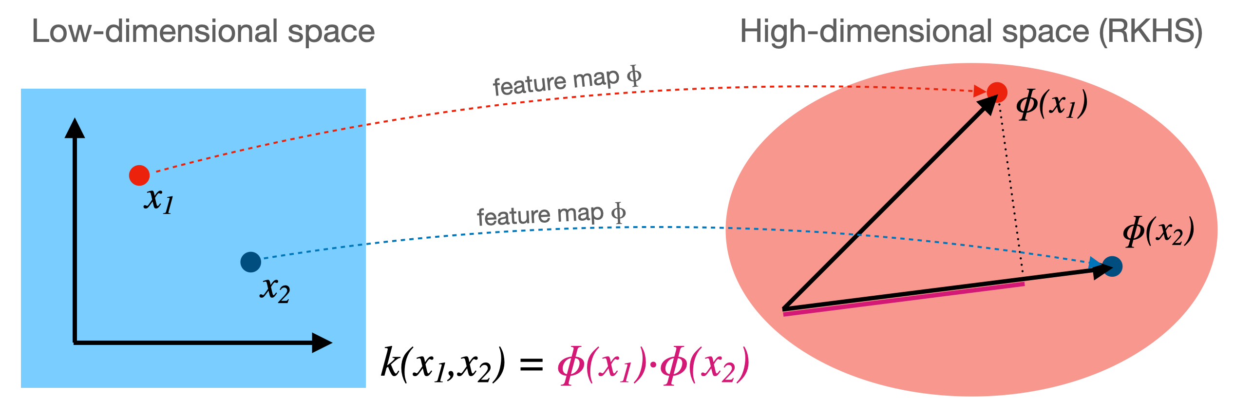
Kernelization

• Kernel $k$ corresponding to a feature map $\Phi$: $ k(\mathbf{x_i},\mathbf{x_j}) = \Phi(\mathbf{x_i}) \cdot \Phi(\mathbf{x_j})$
• Computes dot product between $x_i,x_j$ in a high-dimensional space $\mathcal{H}$
  • Kernels are sometimes called generalized dot products
  • $\mathcal{H}$ is called the reproducing kernel Hilbert space (RKHS)
• The dot product is a measure of the similarity between $x_i,x_j$
  • Hence, a kernel can be seen as a similarity measure for high-dimensional spaces
• If we have a loss function based on dot products $\mathbf{x_i}\cdot\mathbf{x_j}$ it can be kernelized
  • Simply replace the dot products with $k(\mathbf{x_i},\mathbf{x_j})$

Example: SVMs

• Linear SVMs (dual form, for $l$ support vectors with dual coefficients $a_i$ and classes $y_i$): $$\mathcal{L}_{Dual} (a_i) = \sum_{i=1}^{l} a_i - \frac{1}{2} \sum_{i,j=1}^{l} a_i a_j y_i y_j (\mathbf{x_i} . \mathbf{x_j}) $$
• Kernelized SVM, using any existing kernel $k$ we want: $$\mathcal{L}_{Dual} (a_i, k) = \sum_{i=1}^{l} a_i - \frac{1}{2} \sum_{i,j=1}^{l} a_i a_j y_i y_j k(\mathbf{x_i},\mathbf{x_j}) $$

1

Which kernels exist?

• A (Mercer) kernel is any function $k: X \times X \rightarrow \mathbb{R}$ with these properties:

  • Symmetry: $k(\mathbf{x_1},\mathbf{x_2}) = k(\mathbf{x_2},\mathbf{x_1}) \,\,\, \forall \mathbf{x_1},\mathbf{x_2} \in X$
  • Positive definite: the kernel matrix $K$ is positive semi-definite
    • Intuitively, $k(\mathbf{x_1},\mathbf{x_2}) \geq 0$

• The kernel matrix (or Gram matrix) for $n$ points of $x_1,..., x_n \in X$ is defined as:

$$ K = XX^T = \begin{bmatrix} k(\mathbf{x_1}, \mathbf{x_1}) & \ldots & k(\mathbf{x_1}, \mathbf{x_n}) \\ \vdots & \ddots & \vdots \\ k(\mathbf{x_n}, \mathbf{x_1}) & \ldots & k(\mathbf{x_n}, \mathbf{x_n}) \end{bmatrix} $$

• Once computed ($\mathcal{O}(n^2)$), simply lookup $k(\mathbf{x_1}, \mathbf{x_2})$ for any two points
• In practice, you can either supply a kernel function or precompute the kernel matrix

Linear kernel

• Input space is same as output space: $X = \mathcal{H} = \mathbb{R}^d$
• Feature map $\Phi(\mathbf{x}) = \mathbf{x}$
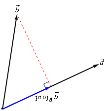
• Kernel: $ k_{linear}(\mathbf{x_i},\mathbf{x_j}) = \mathbf{x_i} \cdot \mathbf{x_j}$
• Geometrically, the dot product is the projection of $\mathbf{x_j}$ on hyperplane defined by $\mathbf{x_i}$
  • Becomes larger if $\mathbf{x_i}$ and $\mathbf{x_j}$ are in the same 'direction'

• Linear kernel between point (0,1) and another unit vector an angle $a$ (in radians)
  • Points with similar angles are deemed similar

Polynomial kernel

• If $k_1$, $k_2$ are kernels, then $\lambda . k_1$ ($\lambda \geq 0$), $k_1 + k_2$, and $k_1 . k_2$ are also kernels
• The polynomial kernel (for degree $d \in \mathbb{N}$) reproduces the polynomial feature map
  • $\gamma$ is a scaling hyperparameter (default $\frac{1}{p}$)
  • $c_0$ is a hyperparameter (default 1) to trade off influence of higher-order terms $$k_{poly}(\mathbf{x_1},\mathbf{x_2}) = (\gamma (\mathbf{x_1} \cdot \mathbf{x_2}) + c_0)^d$$

interactive(children=(IntSlider(value=5, description='degree', max=10, min=1), FloatSlider(value=1.0, descript…

RBF (Gaussian) kernel

• The Radial Basis Function (RBF) feature map builds the Taylor series expansion of $e^x$ $$\Phi(x) = e^{-x^2/2\gamma^2} \Big[ 1, \sqrt{\frac{1}{1!\gamma^2}}x,\sqrt{\frac{1}{2!\gamma^4}}x^2,\sqrt{\frac{1}{3!\gamma^6}}x^3,\ldots\Big]^T$$

• RBF (or Gaussian ) kernel with kernel width $\gamma \geq 0$:
  $$k_{RBF}(\mathbf{x_1},\mathbf{x_2}) = exp(-\gamma ||\mathbf{x_1} - \mathbf{x_2}||^2)$$

interactive(children=(FloatSlider(value=4.91, description='gamma', max=10.0, min=0.01), Output()), _dom_classe…

• The RBF kernel $k_{RBF}(\mathbf{x_1},\mathbf{x_2}) = exp(-\gamma ||\mathbf{x_1} - \mathbf{x_2}||^2)$ does not use a dot product
  • It only considers the distance between $\mathbf{x_1}$ and $\mathbf{x_2}$
  • It's a local kernel : every data point only influences data points nearby
    • linear and polynomial kernels are global : every point affects the whole space
  • Similarity depends on closeness of points and kernel width
    • value goes up for closer points and wider kernels (larger overlap)

interactive(children=(FloatSlider(value=0.5, description='gamma', max=1.0, min=0.1), FloatSlider(value=0.0, de…

Kernelized SVMs in practice

• You can use SVMs with any kernel to learn non-linear decision boundaries

SVM with RBF kernel

• Every support vector locally influences predictions, according to kernel width ($\gamma$)
• The prediction for test point $\mathbf{u}$: sum of the remaining influence of each support vector
  • $f(x) = \sum_{i=1}^{l} a_i y_i k(\mathbf{x_i},\mathbf{u})$

interactive(children=(FloatSlider(value=4.6, description='gamma', max=10.0, min=0.1, step=0.5), FloatSlider(va…

Tuning RBF SVMs

• gamma (kernel width)
  • high values cause narrow Gaussians, more support vectors, overfitting
  • low values cause wide Gaussians, underfitting
• C (cost of margin violations)
  • high values punish margin violations, cause narrow margins, overfitting
  • low values cause wider margins, more support vectors, underfitting

Kernel overview

SVMs in practice

• C and gamma always need to be tuned
  • Interacting regularizers. Find a good C, then finetune gamma
• SVMs expect all features to be approximately on the same scale
  • Data needs to be scaled beforehand
• Allow to learn complex decision boundaries, even with few features
  • Work well on both low- and high dimensional data
  • Especially good at small, high-dimensional data
• Hard to inspect, although support vectors can be inspected
• In sklearn, you can use SVC for classification with a range of kernels
  • SVR for regression

Other kernels

• There are many more possible kernels
• If no kernel function exists, we can still precompute the kernel matrix
  • All you need is some similarity measure, and you can use SVMs
• Text kernels:
  • Word kernels: build a bag-of-words representation of the text (e.g. TFIDF)
    • Kernel is the inner product between these vectors
  • Subsequence kernels: sequences are similar if they share many sub-sequences
    • Build a kernel matrix based on pairwise similarities
• Graph kernels: Same idea (e.g. find common subgraphs to measure similarity)
• These days, deep learning embeddings are more frequently used

The Representer Theorem

• We can kernelize many other loss functions as well

• The Representer Theorem states that if we have a loss function $\mathcal{L}'$ with

  • $\mathcal{L}$ an arbitrary loss function using some function $f$ of the inputs $\mathbf{x}$
  • $\mathcal{R}$ a (non-decreasing) regularization score (e.g. L1 or L2) and constant $\lambda$ $$\mathcal{\mathcal{L}'}(\mathbf{w}) = \mathcal{L}(y,f(\mathbf{x})) + \lambda \mathcal{R} (||\mathbf{w}||)$$

• Then the weights $\mathbf{w}$ can be described as a linear combination of the training samples: $$\mathbf{w} = \sum_{i=1}^{n} a_i y_i f(\mathbf{x_i})$$

• Note that this is exactly what we found for SVMs: $ \mathbf{w} = \sum_{i=1}^{l} a_i y_i \mathbf{\mathbf{x_i}} $
• Hence, we can also kernelize Ridge regression, Logistic regression, Perceptrons, Support Vector Regression, ...

Kernelized Ridge regression

• The linear Ridge regression loss (with $\mathbf{x_0}=1$): $$\mathcal{L}_{Ridge}(\mathbf{w}) = \sum_{i=0}^{n} (y_i-\mathbf{w}\mathbf{x_i})^2 + \lambda \| w \|^2$$
• Filling in $\mathbf{w} = \sum_{i=1}^{n} \alpha_i y_i \mathbf{x_i}$ yields the dual formulation: $$\mathcal{L}_{Ridge}(\mathbf{w}) = \sum_{i=1}^{n} (y_i-\sum_{j=1}^{n} \alpha_j y_j \mathbf{x_i}\mathbf{x_j})^2 + \lambda \sum_{i=1}^{n} \sum_{j=1}^{n} \alpha_i \alpha_j y_i y_j \mathbf{x_i}\mathbf{x_j}$$
• Generalize $\mathbf{x_i}\cdot\mathbf{x_j}$ to $k(\mathbf{x_i},\mathbf{x_j})$ $$\mathcal{L}_{KernelRidge}(\mathbf{\alpha},k) = \sum_{i=1}^{n} (y_i-\sum_{j=1}^{n} \alpha_j y_j k(\mathbf{x_i},\mathbf{x_n}))^2 + \lambda \sum_{i=1}^{n} \sum_{j=1}^{n} \alpha_i \alpha_j y_i y_j k(\mathbf{x_i},\mathbf{x_j})$$

Example of kernelized Ridge

• Prediction (red) is now a linear combination of kernels (blue): $y = \sum_{j=1}^{n} \alpha_j y_j k(\mathbf{x},\mathbf{x_j})$
• We learn a dual coefficient for each point

interactive(children=(FloatSlider(value=1.0, description='gamma', max=2.0, min=0.1), FloatSlider(value=0.0, de…

• Fitting our regression data with KernelRidge

interactive(children=(FloatSlider(value=4.51, description='gamma', max=10.0, min=0.01, step=0.5), Output()), _…

Other kernelized methods

• Same procedure can be done for logistic regression
• For perceptrons, $\alpha \rightarrow \alpha+1$ after every misclassification $$\mathcal{L}_{DualPerceptron}(x_i,k) = max(0,y_i \sum_{j=1}^{n} \alpha_j y_j k(\mathbf{x_j},\mathbf{x_i}))$$
• Support Vector Regression behaves similarly to Kernel Ridge

interactive(children=(FloatSlider(value=4.51, description='gamma', max=10.0, min=0.01, step=0.5), Output()), _…

Summary

• Feature maps $\Phi(x)$ transform features to create a higher-dimensional space
  • Allows learning non-linear functions or boundaries, but very expensive/slow
• For some $\Phi(x)$, we can compute dot products without constructing this space
  • Kernel trick: $k(\mathbf{x_i},\mathbf{x_j}) = \Phi(\mathbf{x_i}) \cdot \Phi(\mathbf{x_j})$
  • Kernel $k$ (generalized dot product) is a measure of similarity between $\mathbf{x_i}$ and $\mathbf{x_j}$
• There are many such kernels
  • Polynomial kernel: $k_{poly}(\mathbf{x_1},\mathbf{x_2}) = (\gamma (\mathbf{x_1} \cdot \mathbf{x_2}) + c_0)^d$
  • RBF (Gaussian) kernel: $k_{RBF}(\mathbf{x_1},\mathbf{x_2}) = exp(-\gamma ||\mathbf{x_1} - \mathbf{x_2}||^2)$
  • A kernel matrix can be precomputed using any similarity measure (e.g. for text, graphs,...)
• Any loss function where inputs appear only as dot products can be kernelized
  • E.g. Linear SVMs: simply replace the dot product with a kernel of choice
• The Representer theorem states which other loss functions can also be kernelized and how
  • Ridge regression, Logistic regression, Perceptrons,...